Source detection and sky model manipulation: PyBDSF and LSMTool 1

Source detection: PyBDSF

Introduction

PyBDSF ( Python Blob Detection and Source Finder) is a Python source-finding software package written by Niruj Mohan, Alexander Usov, and David Rafferty. PyBDSF can process FITS and CASA images and can output source lists in a variety of formats, including makesourcedb (BBS), FITS and ASCII formats. It can be used interactively in a casapy-like shell or in Python scripts. The full PyBDSF manual can be found here.

Setup

The latest version of PyBDSF is installed on the CEP3 cluster. To initialize your environment for PyBDSF, run:

module load pybdsf

After initialization, the interactive PyBDSF shell can be started with the command pybdsf and PyBDSF can be imported into Python scripts with the command import bdsf.

Tutorials

This section gives examples of using PyBDSF on the following: an image that contains only fairly simple sources and no strong artifacts, an image with strong artifacts around bright sources, and an image with complex diffuse emission. It is recommended that interactive mode (enabled with interactive=True) be used for initial runs on a new image, as this allows the user to check the background mean and rms images and the islands found by PyBDSF before proceeding to fitting. Also, if a very large image is being fit, it is often helpful to run on a smaller (but still representative) portion of the image (defined using the trim_box parameter) to verify that the chosen parameters are appropriate before fitting the entire image.

Simple Example

A simple example of using PyBDSF on a LOFAR image (an HBA image of 3C61.1) is shown below. In this case, default values are used for all parameters. Generally, the default values work well on images that contain relatively simple sources with no strong artifacts.

BDSF [1]: inp process_image
BDSF [2]: filename = 'sb48.fits'
BDSF [3]: go
--------> go()
--> Opened 'sb48.fits'
Image size .............................. : (256, 256) pixels
Number of channels ...................... : 1
Beam shape (major, minor, pos angle) .... : (0.002916, 0.002654, -173.36) degrees
Frequency of averaged image ............. : 146.497 MHz
Blank pixels in the image ............... : 0 (0.0%)
Flux from sum of (non-blank) pixels ..... : 29.565 Jy
Derived rms_box (box size, step size) ... : (61, 20) pixels
--> Variation in rms image significant
--> Using 2D map for background rms
--> Variation in mean image significant
--> Using 2D map for background mean
Min/max values of background rms map .... : (0.05358, 0.25376) Jy/beam
Min/max values of background mean map ... : (-0.03656, 0.06190) Jy/beam
--> Expected 5-sigma-clipped false detection rate < fdr_ratio
--> Using sigma-clipping thresholding
Number of islands found ................. : 4
Fitting islands with Gaussians .......... : [====] 4/4
Total number of Gaussians fit to image .. : 12
Total flux in model ..................... : 27.336 Jy
Number of sources formed from Gaussians   : 6

BDSF [4]: show_fit
--------> show_fit()
========================================================================
NOTE -- With the mouse pointer in plot window:
  Press "i" ........ : Get integrated fluxes and mean rms values
                       for the visible portion of the image
  Press "m" ........ : Change min and max scaling values
  Press "0" ........ : Reset scaling to default
  Click Gaussian ... : Print Gaussian and source IDs (zoom_rect mode,
                       toggled with the "zoom" button and indicated in
                       the lower right corner, must be off)
________________________________________________________________________

The figure made by show_fit is shown in Fig. 8.

In the plot window, one can zoom in, save the plot to a file, etc. The list of best-fit Gaussians found by PyBDSF may be written to a file for use in other programs, such as TOPCAT or BBS, as follows:

BDSM [5]: write_catalog
--------> write_catalog()
--> Wrote FITS file 'sb48.pybdsf.srl.fits'

The output Gaussian or source list contains source positions, fluxes, etc. BBS patches are also supported.

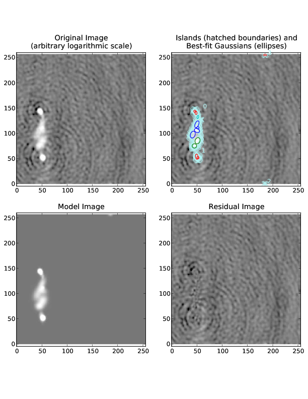
Fig. 8 Output of show_fit, showing the original image with and without sources, the model image, and the residual (original minus model) image. Boundaries of the islands of emission found by PyBDSF are shown in light blue. The fitted Gaussians are shown for each island as ellipses (the sizes of which correspond to the FWHMs of the Gaussians). Gaussians that have been grouped together into a source are shown with the same color. For example, the two red Gaussians of island #1 have been grouped together into one source, and the nine Gaussians of island #0 have been grouped into 4 separate sources. The user can obtain information about a Gaussian by clicking on it. Additionally, with the mouse inside the plot window, the display scaling can be modified by pressing the “m” key, and information about the image flux, model flux, and rms can be obtained by pressing the “i” key.

Image with artifacts

Occasionally, an analysis run with the default parameters does not produce good results. For example, if there are significant deconvolution artifacts in the image, the thresh_isl, thresh_pix, or rms_box parameters might need to be changed to prevent PyBDSF from fitting Gaussians to such artifacts. An example of running PyBDSF with the default parameters on such an image is shown in Fig. 9. It is clear that a number of spurious sources are being detected. Simply raising the threshold for island detection (using the thresh_pix parameter) would remove these sources but would also remove many real but faint sources in regions of low rms. Instead, by setting the rms_box parameter to better match the typical scale over which the artifacts vary significantly, one obtains much better results. In this example, the scale of the regions affected by artifacts is approximately 20 pixels, whereas PyBDSF used a rms_box of 63 pixels when run with the default parameters, resulting in an rms map that is over-smoothed. Therefore, one should set rms_box=(20,10) so that the rms map is computed using a box of 20 pixels in size with a step size of 10 pixels (i.e., the box is moved across the image in 10-pixel steps). See Fig. 11 for a summary of the results of this call.

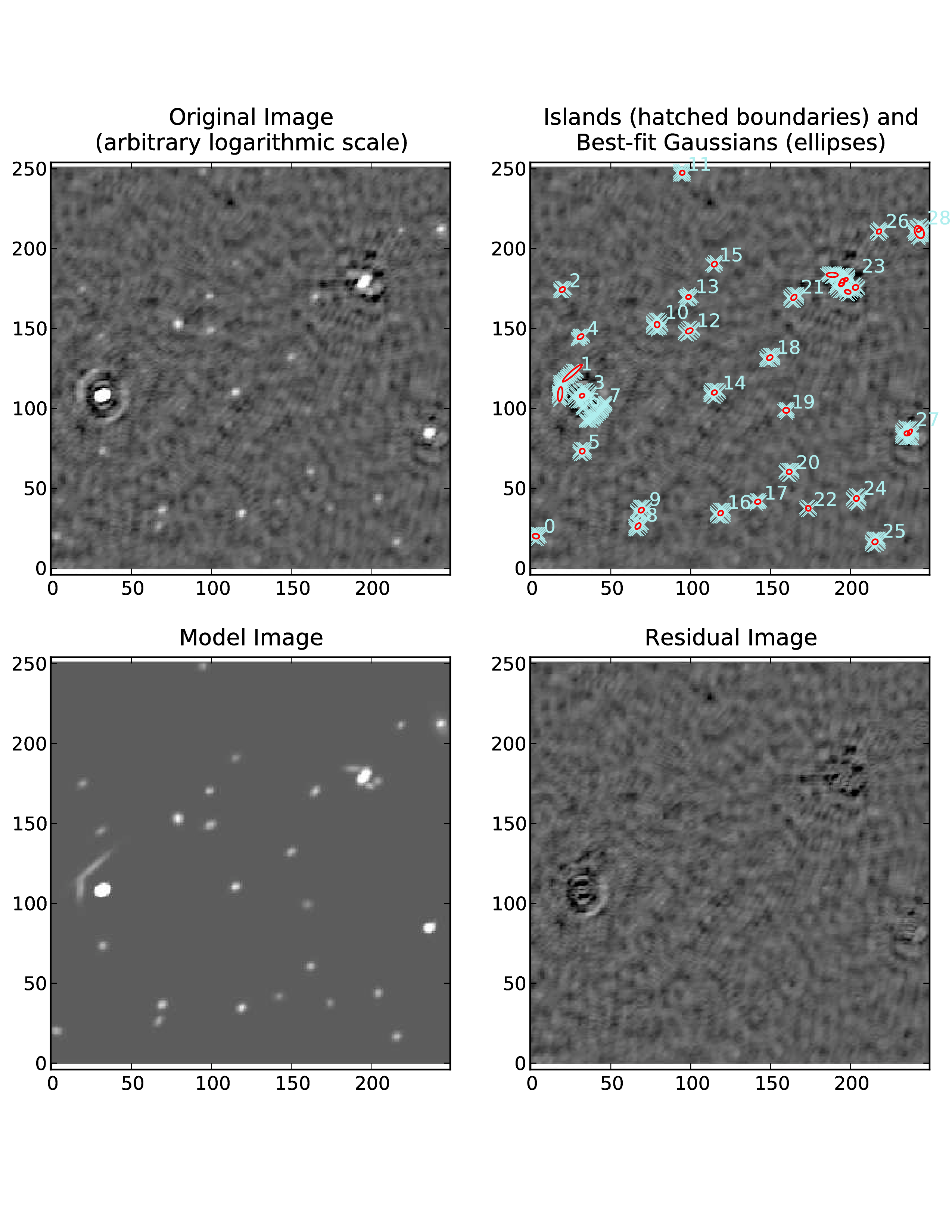
Fig. 9 Example fit with default parameters of an image with strong artifacts around bright sources. A number of artifacts near the bright sources are picked up as sources.

Fig. 10 The background rms map for the same region (produced using show_fit) as in Fig. 9: the rms varies fairly slowly across the image, whereas ideally it would increase more strongly near the bright sources (reflecting the increased rms in those regions due to the artifacts).

Fig. 11 Same as Fig. 9 but with rms_box=(20,10).

Fig. 12 The rms map, corresponding to the fit shown in Fig. 11 varies on scales similar to that of the regions affected by the artifacts, and both bright and faint sources are recovered properly.

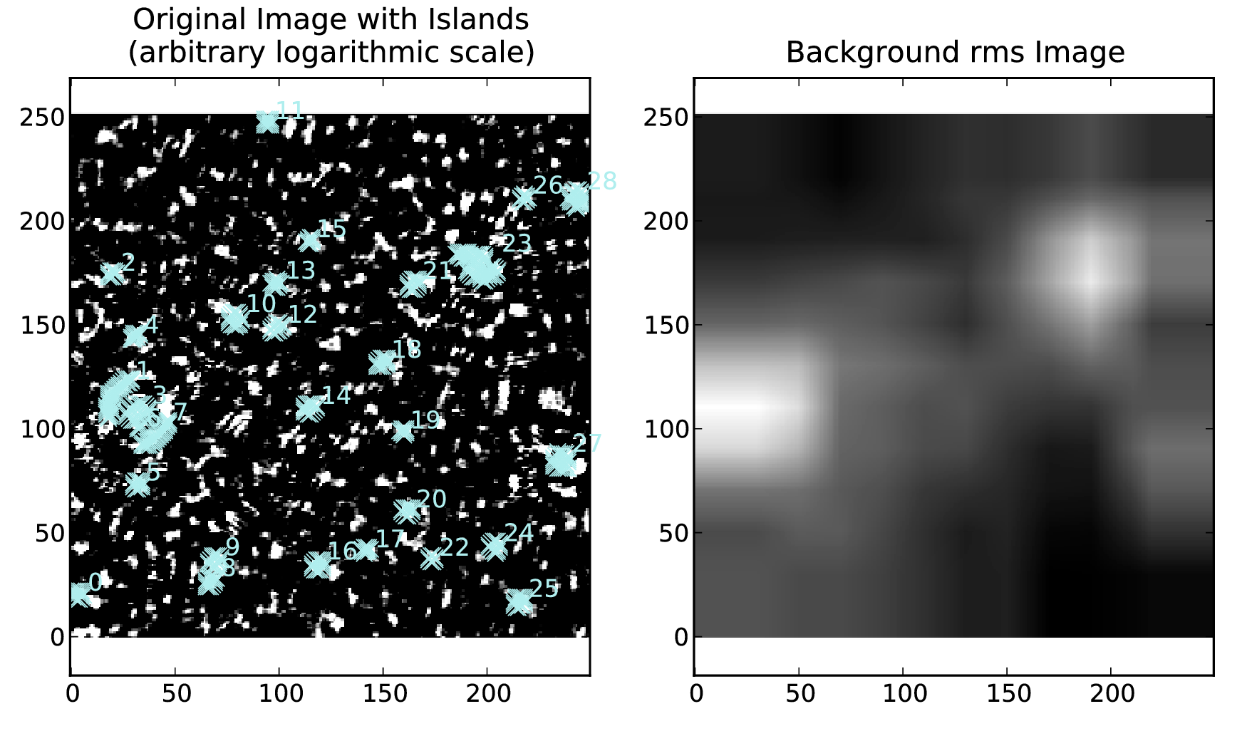
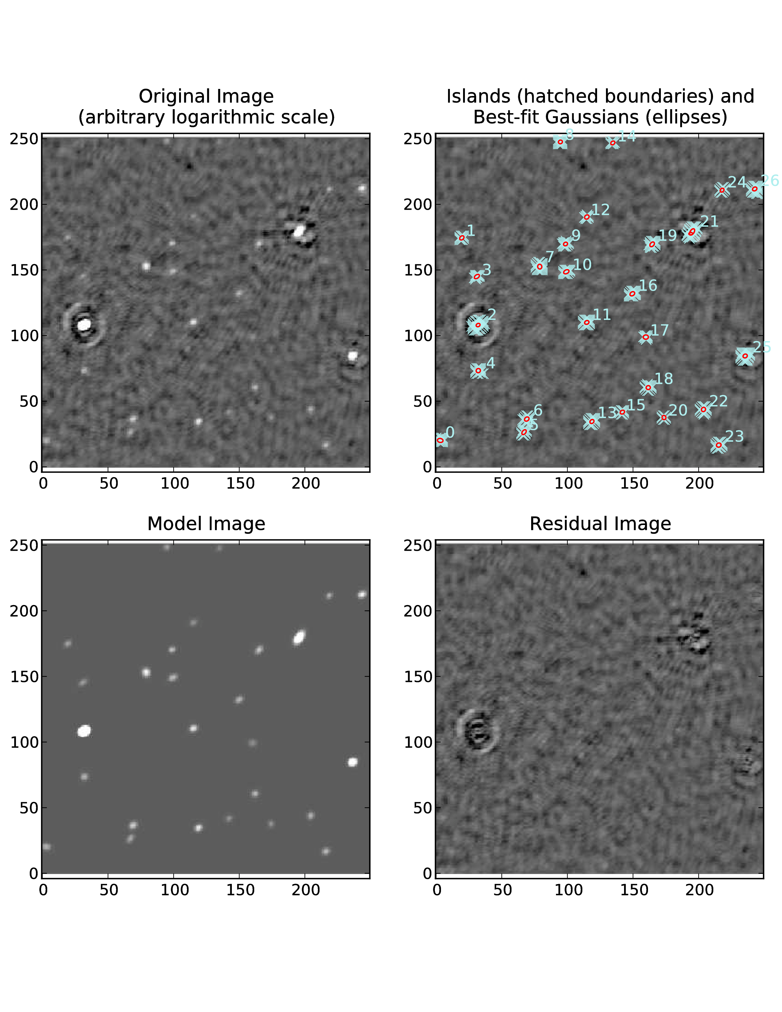
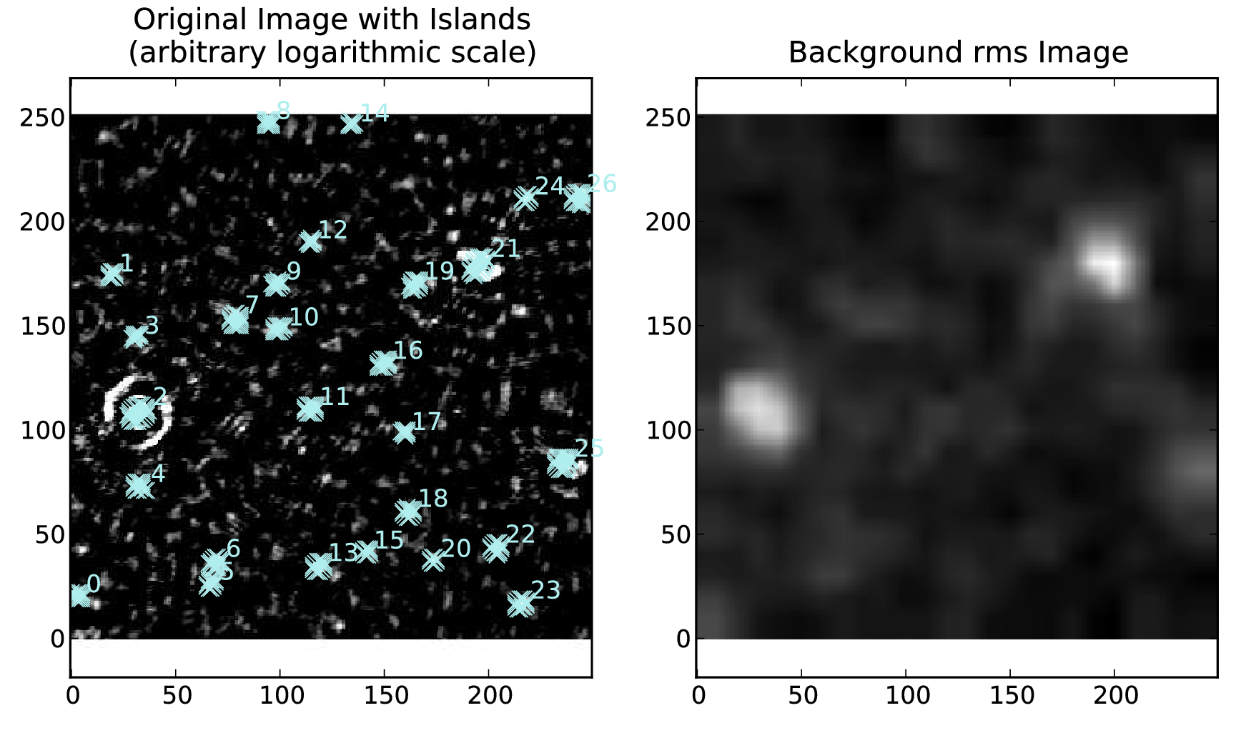
Image with extended emission

If there is extended emission that fills a significant portion of the image, the background rms map will likely be biased high in regions where extended emission is present, affecting the island determination (this can be checked during a run by setting interactive=True). Setting rms_map=False and mean_map=’const’ or ‘zero’ will force PyBDSF to use a constant mean and rms value across the whole image. Additionally, setting atrous_do=True will fit Gaussians of various scales to the residual image to recover extended emission missed in the standard fitting. Depending on the source structure, the thresh_isl and thresh_pix parameters may also have to be adjusted as well to ensure that PyBDSF finds and fits islands of emission properly. An example analysis of an image with significant extended emission is shown in Fig. 13.

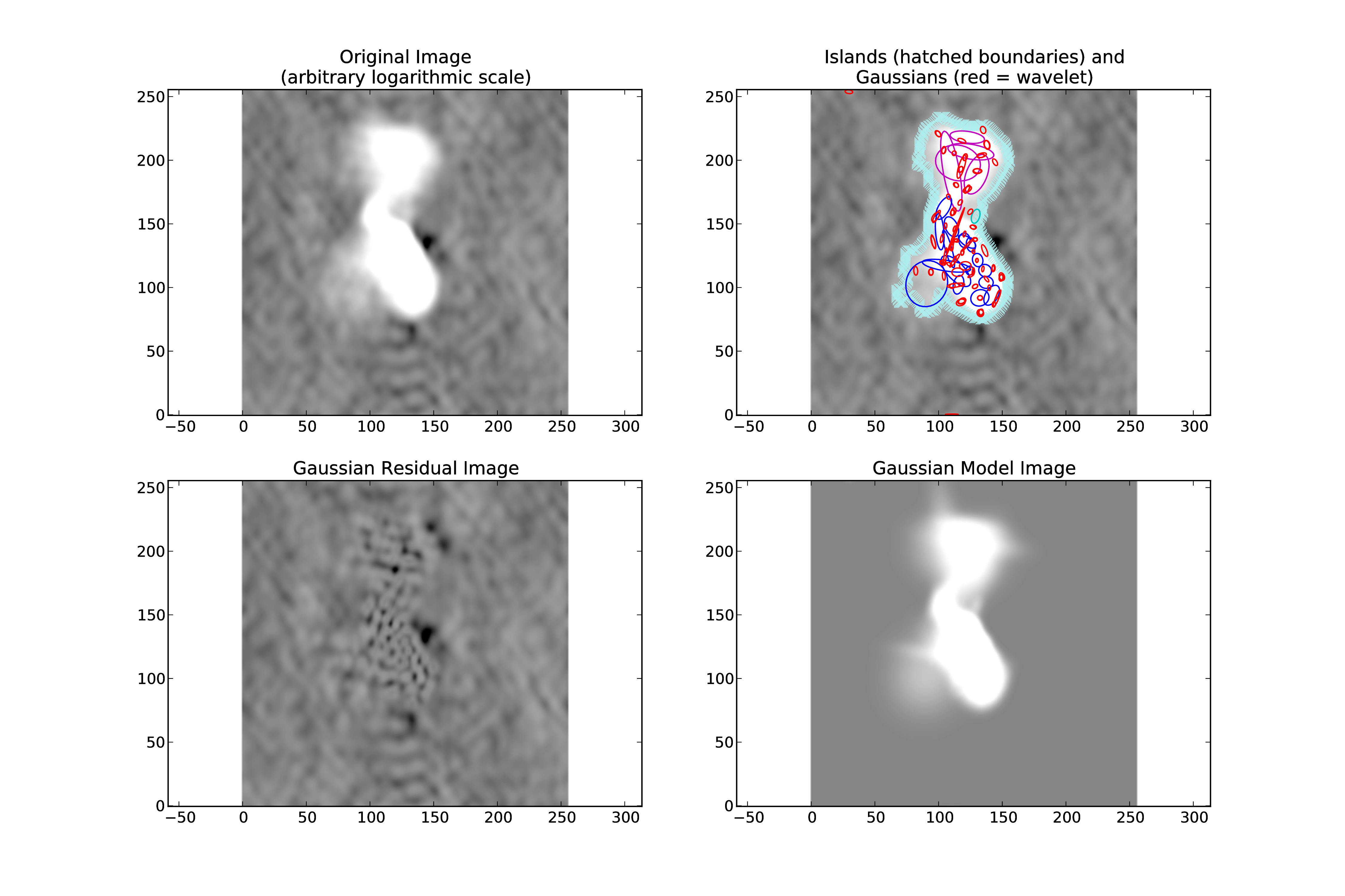
Fig. 13 Example fit of an image of Hydra A with rms_map=False, mean_map=’zero’, and atrous_do=True. The values of thresh_isl and thresh_pix were adjusted before fitting (by setting interactive=True) to obtain an island that enclosed all significant emission.

Usage in python scripts

PyBDSF may also be used non-interactively in Python scripts (for example, to automate source detection in a large number of images for which the optimal analysis parameters are known). To use PyBDSF in a Python script, import it by calling from lofar import bdsm inside your script. Processing may then be done using bdsm.process_image() as follows:

img = bdsm.process_image(filename, <args>)

where filename is the name of the image (in FITS or CASA format) or PyBDSF parameter save file and <args> is a comma-separated list of arguments defined as in the interactive environment (e.g., beam = (0.033, 0.033, 0.0), rms_map=False). If the fit is successful, PyBDSF will return an “Image” object (in this example named “img”) which contains the results of the fit (among many other things). The same tasks used in the interactive PyBDSF shell are available for examining the fit and writing out the source list, residual image, etc. These tasks are methods of the Image object returned by bdsm.process_image() and are described below:

• img.show_fit(): This method shows a quick summary of the fit by plotting the input image with the islands and Gaussians found, along with the model and residual images.

• img.export_image(): Write an internally derived image (e.g., the model image) to a FITS file.

• img.write_catalog(): This method writes the Gaussian or source list to a file.

The input parameters to each of these tasks are the same as those available in the interactive shell. For more details and scripting examples, see PyBDSF documentation.

Sky model manipulation: LSMTool

Introduction

LSMTool is a Python package which allows for the manipulation of sky models in the makesourcedb format (used by BBS and DPPP). Such models include those output by PyBDSF, those made by gsm.py, and CASA clean-component models (after conversion with casapy2bbs.py). The full LSMTool manual is located at http://www.astron.nl/citt/lsmtool.

Setup

To initialize your environment for LSMTool, users on the CEP3 cluster should run the following command:

module load lsmtool

Tutorials

This section gives examples of using LSMTool to select sources and group them into patches.

Filter and Group a Sky Model

As with many of the LOFAR tools (e.g., DPPP), LSMTool can be run with a parset that specifies the operations to perform and their parameters. Below is an example parset that filters on the Stokes I flux density (selecting only those sources with flux densities above 1 mJy), adds a source to the sky model, and then groups the sources into patches (so that each patch has a total flux density of around 50 Jy):

LSMTool.Steps = [selectbright, addsrc, grp, setpos]

 # Select only sources above 1 mJy
 LSMTool.Steps.selectbright.Operation = SELECT
 LSMTool.Steps.selectbright.FilterExpression = I > 1.0 mJy

 # Add a source
 LSMTool.Steps.addsrc.Operation = ADD
 LSMTool.Steps.addsrc.Name = new_source
 LSMTool.Steps.addsrc.Type = POINT
 LSMTool.Steps.addsrc.Ra = 277.4232
 LSMTool.Steps.addsrc.Dec = 48.3689
 LSMTool.Steps.addsrc.I = 0.69

 # Group using tessellation to a target flux of 50 Jy
 LSMTool.Steps.grp.Operation = GROUP
 LSMTool.Steps.grp.Algorithm = tessellate
 LSMTool.Steps.grp.TargetFlux = 50.0 Jy
 LSMTool.Steps.grp.Method = mid

 # Set the patch positions to their midpoint and write final skymodel
 LSMTool.Steps.setpos.Operation = SETPATCHPOSITIONS
 LSMTool.Steps.setpos.Method = mid
 LSMTool.Steps.setpos.OutFile = grouped.sky

In the first line of this parset the step names are defined. Steps are applied sequentially, in the same order defined in the list of steps. See the full manual for a list of steps and their allowed parameters.

LSMTool can also be used interactively (in IPython, for example) or in Python scripts without the need for a parset, which is generally more convenient. To use LSMTool in a Python script or interpreter, import it as follows:

>>> import lsmtool

A sky model can then be loaded with, e.g.:

>>> s = lsmtool.load('skymodel.sky')

The following commands duplicate the steps done using the parset above:

# Select only sources above 1 mJy
 >>> s.select('I > 1.0 mJy')

 # Add a source
 >>> s.add({'Name':'new_source', 'Type':'POINT', 'Ra':277.4232, 'Dec':48.3689, 'I':0.69})

 # Group using tessellation to a target flux of 50 Jy
 >>> s.group(algorithm='tesselate', targetFlux='10.0 Jy')

 # Set the patch positions to their midpoint and write final skymodel
 >>> s.setPatchPositions(method='mid')
 >>> s.write('grouped.sky')

Select sources within a given region

In this example, LSMTool is used to select only those sources within a radius of 1 degree of a given position (RA = 123.2123 deg, Dec = +34.3212 deg):

# Get the distance of each source to the given position (here specified as
# RA, Dec in degrees; one can also specify the postion in makesourcedb format)
>>> dist = s.getDistance(123.2123, 34.3212)

# Remove sources with distances of more than 1 degree
>>> s.remove(dist > 1.0)

Find Sources below a Given Size in a Clean-component Sky Model

It can be difficult to identify sources in a clean-component sky model (such as one made by casapy2bbs.py), as there is no explicit connection between the components. LSMTool provides a grouping algorithm (named threshold) that can be used to find sources in such a sky model. For example, the following lines will identify sources and select only those smaller than 3 arcmin:

# Use thresholding to group clean components into patches by smoothing the
# clean-component model with a Gaussian of 60 arcsec FWHM
>>> s.group('threshold', FWHM='60.0 arcsec')

# Get the sizes (in arcmin) of the patches, weighted by the clean-component
# fluxes
>>> sizes = s.getPatchSizes(units='arcmin', weight=True)

# Select sources with sizes below 3 arcmin (the "aggregate" parameter means
# to select on the patch sizes instead of the individual source sizes)
>>> s.select(sizes < 3.0, aggregate=True)

Footnotes

1

This section is maintained by David Rafferty).