Sky Model Construction Using Shapelets 1 ¶

In this chapter, we give a tutorial overview of sky model construction using shapelets and other source types suitable for self calibration. Note that shapelets decomposition should be used in the case we are dealing with extended sources.

Introduction¶

In this tutorial, we present construction of accurate and efficient sky models for calibration of LOFAR data, using shapelets. However, we do not present any theoretical material on shapelets and their strengths and weaknesses for use in self calibration. We refer the reader to Yatawatta (2010; 2011) for a more mathematical presentation on these subjects.

We always work with FITS images for our model construction. Therefore, it is assumed that you already have an image of the sky that is being observed, which is good enough to create a sky model from. You can obtain a FITS image of the sky that is being observed in many ways. For example, you can use images made by other instruments (at a probably different frequency/resolution) and one such source is Sky View. You can also do a rough calibration of the data and make a preliminary image of the sky. And if you are hardcore, you can also manipulate an empty FITS file to create the shape that you want to model (we shall discuss this later).

The FITS file contains more information than that is shown as the image. Since we are dealing with images made with radio interferometers, almost all images have been deconvolved (e.g. by CLEAN). The Point Spread Function (PSF) plays an important role in deconvolution. Most FITS files have information about the approximate PSF that we will be using a lot. This information is stored in the header of the FITS file with the keywords BMAJ, BMIN, and BPA. The BMAJ and BMIN keywords give the PSF width as the major and minor axes of a Gaussian. The BPA keyword gives the position angle (or the rotation) of the Gaussian. We will learn how to manipulate these keywords (or add them if your FITS file is without them) later.

Throughout this tutorial, we will calibrate an observation of Virgo-A around 50 MHz. In Fig. ref{shp:viravla}, we have shown an image of Virgo-A made by the VLA at 74 MHz. The red circle on top right corner shows the PSF for this image. Although the frequency and resolution does not match the LOFAR observation, we will be using this image to build a sky model.

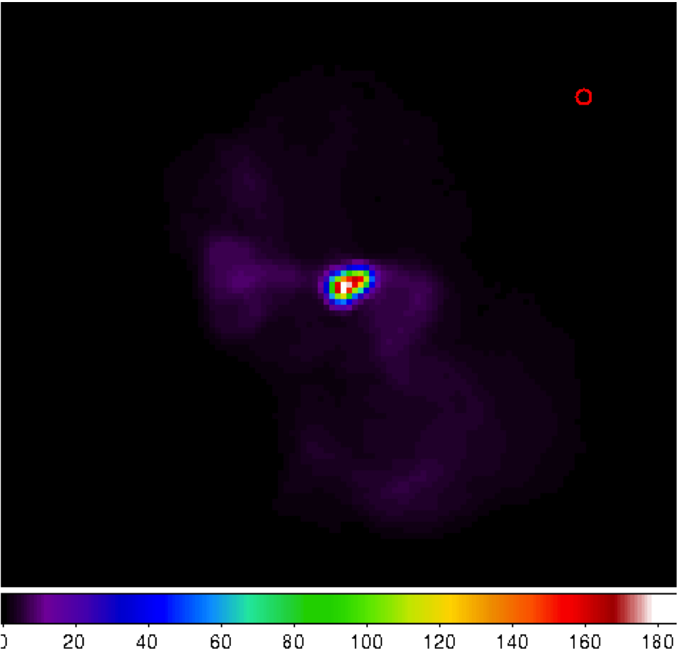
Fig. 26 Virgo-A image made by the VLA at 74 MHz. The red circle on top right corner is the PSF.¶

Looking closer at Fig. 26, we see that there is bright compact structure at the center and weak diffuse structure surrounding it. You should always keep in mind the golden rule in source modeling: A point source is best modeled by a point source and nothing else. Almost always, you will have images with both compact structure (best modeled by point sources) and extended structure (best modeled using shapelets). In our example, we need to model the central compact structure as point sources and the remainder as shapelets. See Yatawatta (2010) for a theoretical explanation.

Software overview¶

There are several steps needed in building a good sky model. You can skip some steps depending on particular requirements (and if you can use other software to do the same). We give a general overview of various tools used in different stages of sky model construction. All the software is installed in /opt/cep/shapelet/bin in the CEP clusters.

modkey¶

The program modkey is used to modify keywords in FITS files. For example, if you want to modify the BMAJ keyword in the example.fits FITS file

modkey -f example.fits -k BMAJ -d 0.1

will set the value of BMAJ to \(0.1\). If this key does not exist, it will be created. Try using

modkey -h

for more usage examples.

fitscopy¶

Most FITS files will be too large to work with. The sources that you want to model will be only in small areas of the large FITS file. The program fitscopy will create a smaller FITS file by selecting a smaller rectangle from the larger FITS file. For example, if you want to select the area given by the pixels \([x0,y0]\) bottom left hand corner and \([x1,y1]\) top right hand corner of the file large.fits

fitscopy large.fits small.fits x0 y0 x1 y1

will do the trick.

ds9 and kvis¶

We use both ds9 and kvis to display FITS file as well as display regions (ds9) and annotations (kvis).

Duchamp¶

The source extraction program Duchamp is written by Matthew Whiting. We will only be using Duchamp to create a mask file for a given FITS image. A mask is a FITS file with the same size as the original image, but with zeros everywhere except at the selected pixels. Here is a simple configuration file for creating a mask for example.fits FITS file

##########################################
imageFile example.fits
logFile         logfile.txt
outFile         results.txt
spectraFile     spectra.ps
minPix          5
flagATrous      0
snrRecon        10.
snrCut          5.
threshold 0.030
minChannels     3
flagBaseline    0
flagKarma 1
karmaFile duchamp.ann
flagnegative 0
flagMaps 0
flagOutputMask 1
flagMaskWithObjectNum 1
flagXOutput 0
############################################

The threshold for pixel selection is given by the threshold parameter which is \(0.03\) in the above example. After creating the configuration file, and saving it as myconf.txt, you can run Duchamp as

Duchamp -p myconf.txt

This will create a mask file called example.MASK.fits which we will be using at later stages.

NOTE: Only versions later than 1.1.9 produce the right output.

buildsky¶

We mentioned before that whenever we have compact structure, it is best modeled by using point sources. The program buildsky creates a model with only point sources for a given image. However, we must have a mask file. So if we have example.fits image and example.MASK.fits mask file, the simplest way of using this is

buildsky -f example.fits -m example.MASK.fits

This will create a file called example.fits.sky.txt that can be used as input for BBS. It also creates a ds9 region file called example.fits.ds9.reg that you can use to check your sky model.

You can see other options by typing

buildsky -h

restore¶

We use restore to restore a sky model onto a FITS file. The sky model can be specified in two different ways. It can directly read a BBS sky model like

# Name, Type, Ra, Dec, I, Q, U, V, MajorAxis, MinorAxis, Orientation,
# ReferenceFrequency, SpectralIndex= with '[]'
# NOTE: no default values taken, for point sources
#  major,minor,orientation has to be all zero
# Example:
# note: bmaj,bmin, Gaussian radius in degrees, bpa also in degrees
Gtest1, GAUSSIAN, 18:59:16.309, -22.46.26.616, 100, 100, 100, 100, 0.222, 0.111, 100, 150e6, [-1.0]
Ptest2, POINT, 18:59:20.309, -22.53.16.616, 100, 100, 100, 100, 0, 0, 0, 140e6, [-2.100]

and also it can read an LSM sky model like (see chapter on SAGECAL for more information)

## this is an LSM text (hms/dms) file
## fields are (where h:m:s is RA, d:m:s is Dec):
## name h m s d m s I Q U V spectral_index RM
##    extent_X(rad) extent_Y(rad) pos_angle(rad) freq0
P1C1 1 35 29.128 84 21 51.699 0.061585 0 0 0 0 0 0 0 0 1000000.0

using -o 0 for BBS and -o 1 or -o 1 for LSM. Note that buildsky will now (version 0.0.6) only produce LSM with 3rd order spectra. Spectral indices use natural logarithm, \(\exp(\ln(I_0) + p1*\ln(f/f_0) + p2*\ln(f/f_0)^2 + \ldots)\) so if you have a model with common logarithms like

\[10^{(\log(J_0) + q1*\log(f/f_0) + q2*\log(f/f_0)^2 + \ldots)}\]

then, conversion is \(I_0=J_0\), \(p1=q1\), \(p2=q2/\ln(10)\), \(p3=q3/(\ln(10)^2)\) and so on.

As you can see, both above sky models are the same. In addition, the LSM sky model can be used to represent Gaussians (name starting with G), disks (name starting with D) and rings (name starting with R).

Once you have such a sky model (text file sky.txt), and a FITS file called example.fits, you can do many things

restore -f example.fits -i sky.txt

will replace the FITS file with the sky model, so the original image will be overwritten;

restore -f example.fits -i sky.txt  -a

will add the sky model to the image; and

restore -f example.fits -i sky.txt  -s

will subtract the sky model from the FITS file.

You can also use solutions obtained by SAGECal when you restore a sky model:

restore -f example.fits -i sky.txt -c sagecal_cluster.txt -l sagecal_sky.txt

will use the solution file sagecal_sky.txt and the cluster file sagecal_cluster.txt while restoring the sky model. New solution files created by SAGECal has 3 additional lines at the beginning. Newer versions (0.0.10) of restore will properly handle this.

As before, you can see more options by typing

restore -h

shapelet_gui¶

The GUI used in decomposing FITS file to shapelets is called shapelet_gui. Once you run this program you will be seeing the GUI as in Fig. 27.

Fig. 27 The shapelet_gui initial screen.¶

The essential parameters can be changed by using View->Change Options menu item. Once you select this, you will see the dialog as in Fig. 28.

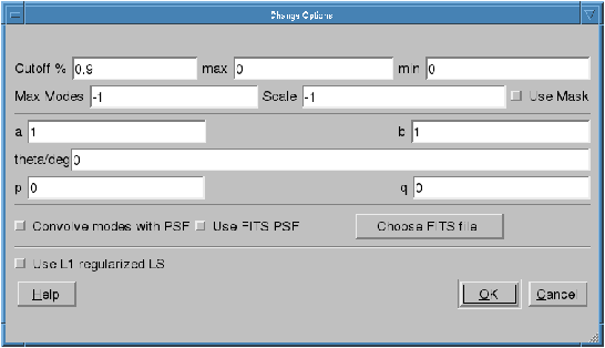
Fig. 28 The options dialog for shapelet decomposition.¶

We will go through the options in Fig. ref{shp:gui1} one by one.

Cutoff This parameter is used to select the rectangle of pixels where most of the flux in the image is concentrated. A cutoff of \(0.9\) will select all the pixels above \(0.1\) of the peak flux. By using cutoff of \(1.0\), the whole image is selected.
max If this value is not \(0\), pixels above this value will be truncated to this value.
min If this value is not \(0\), pixels below this value will be truncated to \(0\).
Max Modes The maximum number of shapelet basis functions used. If you enter \(100\) here, a \(10\times10\) array of shapelet modes will be used. Use a small number here to save memory. The default value of \(-1\) makes the program determine this automatically.
Scale This is the scale (or \(\beta\)) of the shapelet basis. The default value of \(-1\) makes the program determine this automatically.
Use Mask Instead of using a cutoff, we can also use a mask to select the pixels for shapelet modeling. The mask can be created using Duchamp. If this option is enabled, for the image example.fits FITS file, you must have the example.MASK.fits mask file in the same location. Note: make sure that flagMaskWithObjectNum 0 is used for the input for Duchamp.
a, b, theta These parameters are used in linear transforms. It is possible to scale and rotate your image before you do a shapelet decomposition. This is not yet implemented in BBS.
p, q Normally, the center of the shapelet basis is selected to be the center of the FITS file. However, you can give any arbitrary location of your FITS file as the center by changing p and q. These have to be in pixels.
Convolve modes with PSF As we mentioned before, almost all images will have a PSF. If the PSF is larger than the pixel size, it is useful to enable this option. The PSF is obtained by using the BMAJ, BMIN, BPA keywords of the FITS file.
Use FITS PSF It is also possible to give another FITS file as the PSF. This generally has to be much smaller than the image.
Use L1 regularized LS Instead of using normal L2 minimization to find the shapelet decomposition, you can also use L1 regularization. The difference in results is negligible in most cases.

It is advised to always enable Use Mask and Convolve modes with PSF options to get best performance. You can also get more information on all these options by clicking the Help button.

Finally, after fine tuning your options, you can select File->Open to select your FITS file and it will produce an output like Fig. 29. If you are not satisfied with the result, you can go back and View->Change Options to re-tune your parameters. Once you have done that, you can decompose the same FITS file by selecting View->Decompose from the menu.

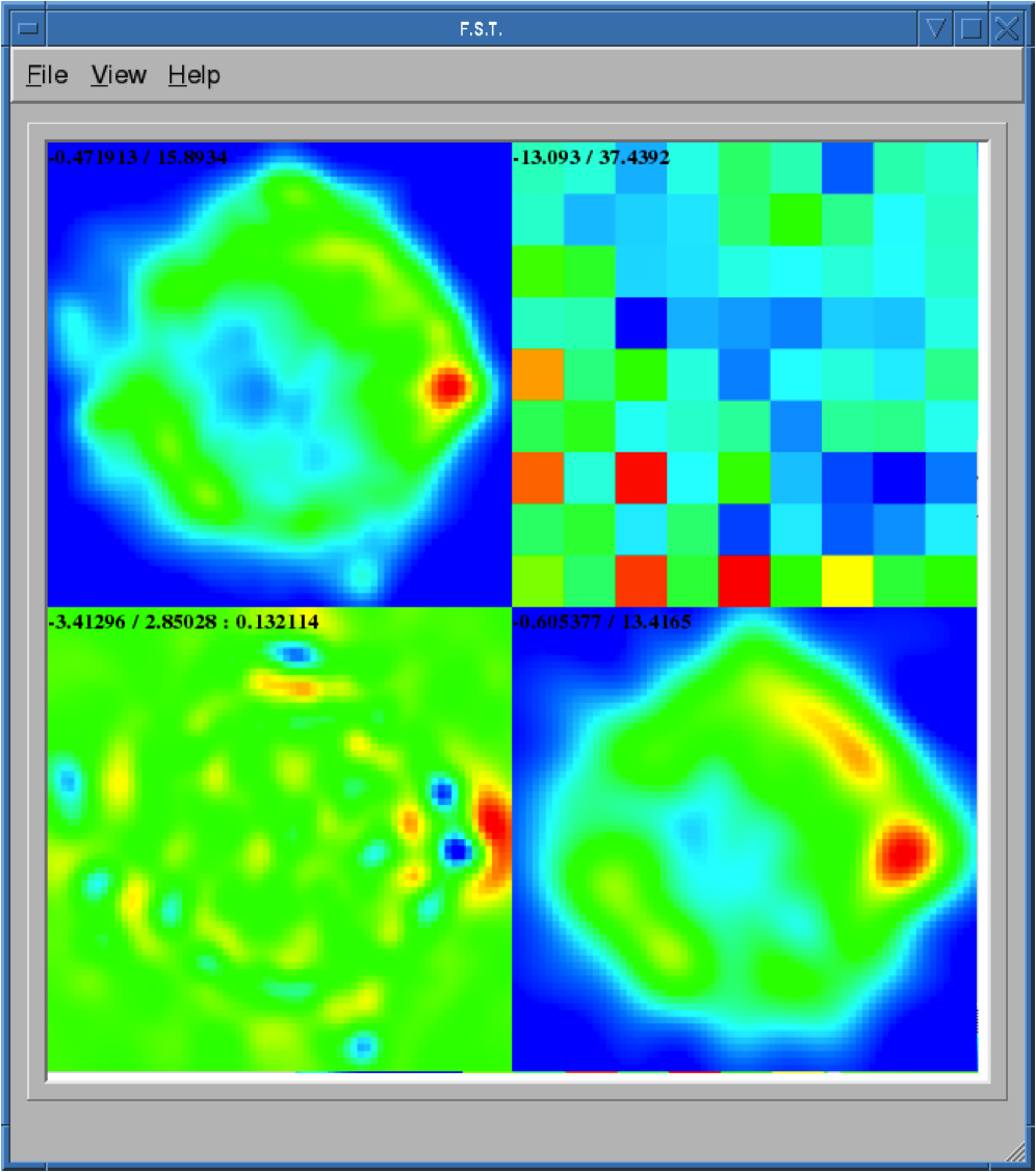
Fig. 29 Output of shapelet modelling: (top left) original image (top right) shapelet modes (bottom left) residual image (bottom right) shapelet model.¶

Apart from displaying the output, each time you decompose a FITS file, shapelet_gui will produce several files. Most importantly, for your input example.fits image, it will produce example.fits.modes text file that can be used in BBS. Here is an extract of one such file:

23 27.273176 58 49 1.217289
1.255970e-03
1.864041e+01
5.311269e+00
3.354807e+01
7.081891e+00
3.743916e+01
1.209364e+01
2.458361e+01
7.033823e+00
8.411157e+00
-- many more rows --
# BBS format:
## NAME shapelet  23:23:27.273176 58.49.1.217289 1.0 thisfile.fits.modes

The thing to note from the above listing is the last line. It shows you exactly how to enter this into BBS. You have to create a text file such as

#
FORMAT = Name Type RA Dec I IShapelet

Ex1 shapelet  23:23:27.273176 58.49.1.217289 1.0 example.fits.modes

where we have copied the last line, changing the source name to whatever we like (in this case Ex1) and changing the last field to example.fits.modes.

convert_skymodel.py¶

This script converts sky models in BBS format to LSM format and vice versa.

Usage: convert_skymodel.py [options]

Options:
  -h, --help            show this help message and exit
  -i INFILE, --infile=INFILE
                        Input sky model
  -o OUTFILE, --outfile=OUTFILE
                        Output sky model (overwritten!)
  -b, --bbstolsm        BBS to LSM
  -l, --lsmtobbs        LSM to BBS

create_clusters.py¶

This script creates a cluster file that can be used by SAGECal, given an input sky model.

Usage: create_clusters.py [options]

Options:
  -h, --help            show this help message and exit
  -s SKYMODEL, --skymodel=SKYMODEL
                        Input sky model
  -c CLUSTERS, --clusters=CLUSTERS
                        Number of clusters
  -o OUTFILE, --outfile=OUTFILE
                        Output cluster file
  -i ITERATIONS, --iterations=ITERATIONS
                        Number of iterations

The sky model has to be in LSM format, -c option gives the number of clusters to create. It uses weighted K-means clustering algorithm, and the number of iterations for this is given by -i, usually about 10 iterations is enough for convergence. This and many other scripts can be downloaded from sagecal.sf.net.

Step by Step Example¶

In this section, we will use most of the programs described before to calibrate a LOFAR observation of Virgo-A. We will use Fig. 26 (FITS file vira-cen.fits) to build the initial sky model.

Initial point source model¶

As we mentioned in the Introduction, the central compact part in Fig. 26 is best modeled using point sources. Therefore, we create the following as input to Duchamp

imageFile vira-cen.fits
logFile   logfile.txt
outFile   results.txt
spectraFile spectra.ps
minPix    5
flagATrous  0
snrRecon  10.
snrCut    5.
threshold 10.010
minChannels 3
flagBaseline    0
flagKarma 1
karmaFile duchamp.ann
flagnegative 0
flagMaps 0
flagOutputMask 1
flagMaskWithObjectNum 1
flagXOutput 0

After running Duchamp with this input file, we select only the bright compact center (that is the reason for using \(10.01\) as threshold) as seen on Fig. 26.

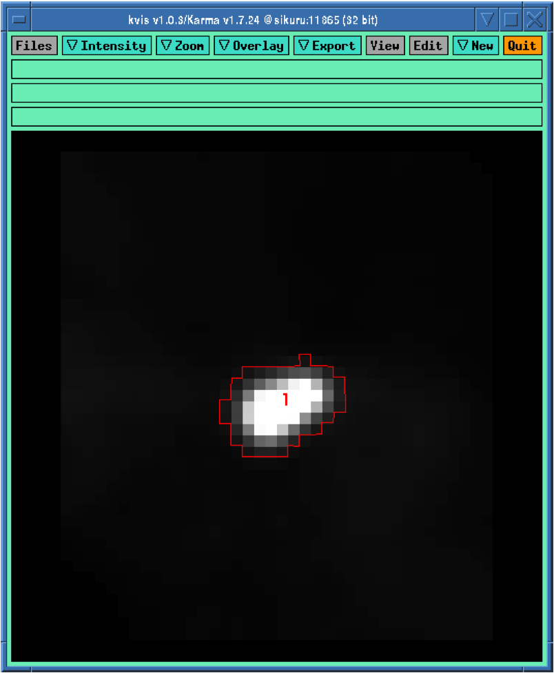
Fig. 30 Compact center indicated by the red curve.¶

Now we run buildsky to build the sky model for this as

buildsky -f vira-cen.fits -m vira-cen.MASK.fits

This will create the first part of the sky model for BBS (file vira-cen.fits.sky.txt):

   # (Name, Type, Ra, Dec, I, Q, U, V,
ReferenceFrequency='60e6', SpectralIndexDegree='0',
SpectralIndex:0='0.0', MajorAxis, MinorAxis, Orientation) = format
 # The above line defines the field order and is required.
 P1C1, POINT, 12:30:45.93, +12.23.48.07, 172.155091, 0.0, 0.0, 0.0
 P1C2, POINT, 12:30:47.39, +12.23.51.92, 141.518663, 0.0, 0.0, 0.0
 P1C3, POINT, 12:30:47.34, +12.23.31.64, 173.054910, 0.0, 0.0, 0.0
 P1C4, POINT, 12:30:48.90, +12.23.40.67, 177.304557, 0.0, 0.0, 0.0
 P1C5, POINT, 12:30:48.75, +12.23.21.23, 155.029319, 0.0, 0.0, 0.0

Using ds9 we can also see our sky model as in Fig. 31.

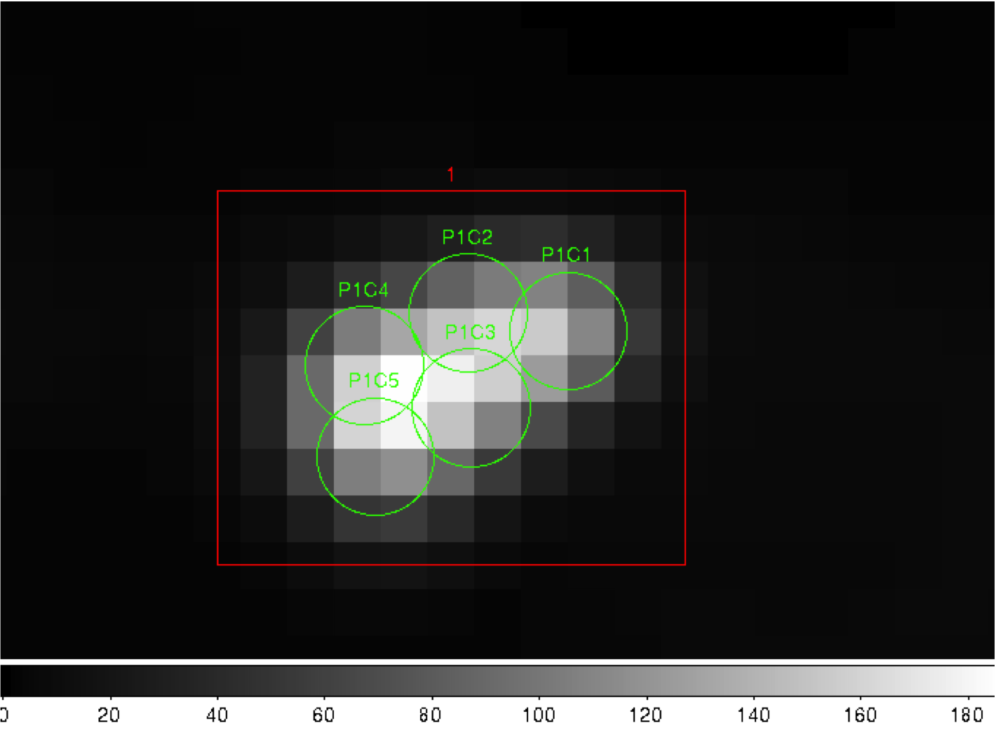
Fig. 31 Compact center modeled by two point sources (green circles).¶

Initial shaplet model¶

Next, we need to model the extended structure in Fig. 26. However, before we do this we have to subtract our point source model from this figure. We use restore to do this

restore -f vira-cen.fits -i vira-cen.fits.sky.txt -s

which gives us the new image as in Fig. 32.

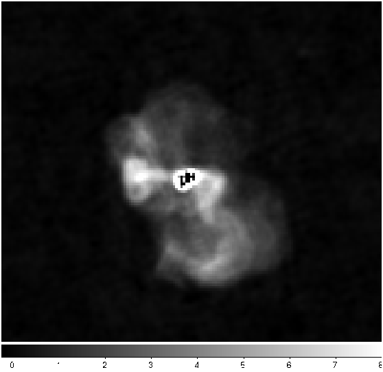
Fig. 32 Diffused structure after subtracting the center.¶

Note that the bright central part in Fig. 32 is almost subtracted. It is not completely gone, and some parts of it is negative. Nevertheless, this is all right for now because we are only building an approximate sky model. Now we need to create another mask for this image for the diffused structure. We use to following file for Duchamp.

imageFile vira-cen.fits
logFile   logfile.txt
outFile   results.txt
spectraFile spectra.ps
minPix    5
flagATrous  0
snrRecon  10.
snrCut    5.
threshold 1.010
minChannels 3
flagBaseline    0
flagKarma 1
karmaFile duchamp.ann
flagnegative 0
flagMaps 0
flagOutputMask 1
flagMaskWithObjectNum 0
flagXOutput 0

Note that we have used a lower threshold (\(1.01\)) this time, compared to the previous value. Once running Duchamp, we get the mask as indicated by Fig. 33.

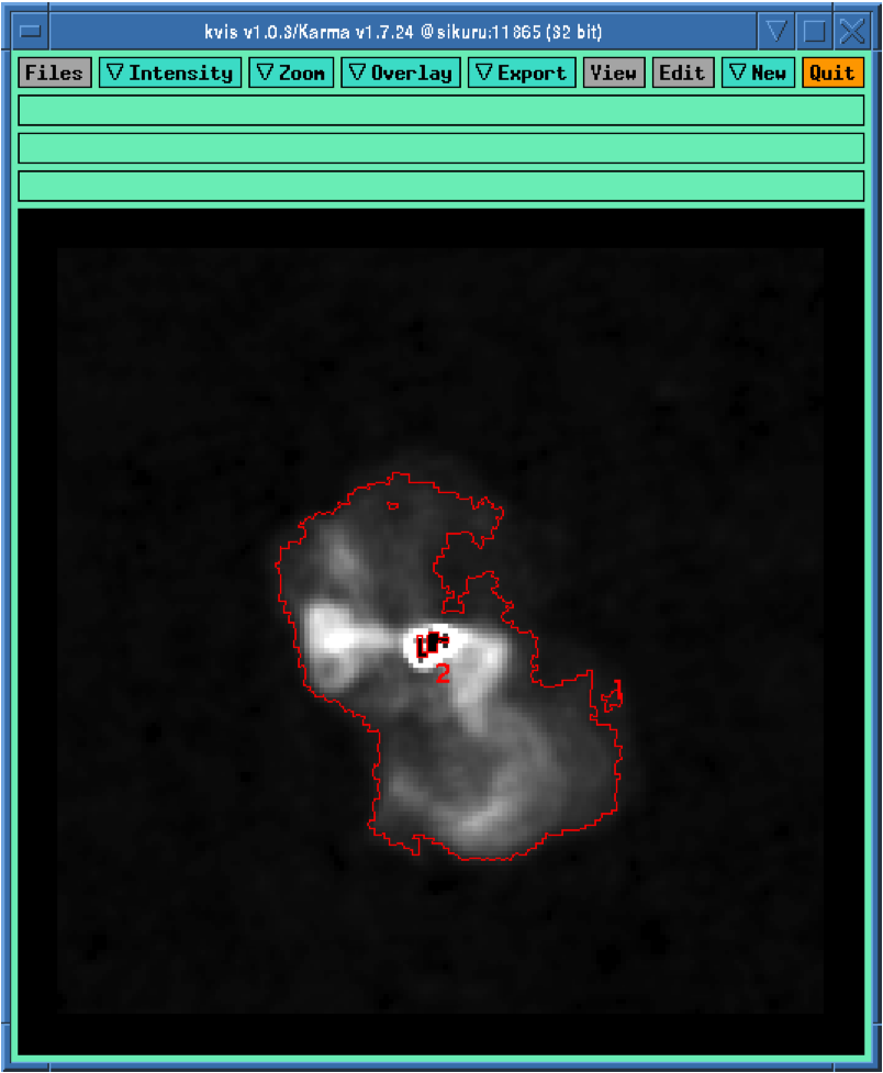
Fig. 33 Mask for the diffused structure.¶

Now we are ready to build the shapelet model. We first change some parameters using View->Change Options. We set Cutoff to \(1.0\), Max Modes to \(200\), and the center p to 75 and q to 74 to move the origin of the shapelets a bit. Furthermore, we enable Use Mask and Convolve Modes with PSF options. Then we use File->Open to select vira-cen.fits as input. After a few seconds, we get the result as in Fig. 34.

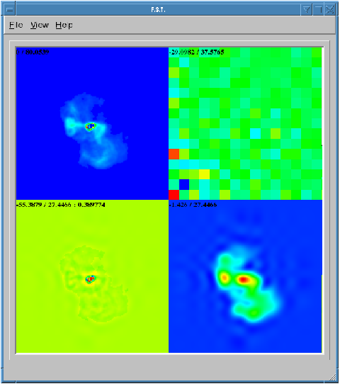
Fig. 34 Shapelet model of the diffused structure.¶

We can easily create an input to BBS for this shapelet model as follows:

#
FORMAT = Name Type RA Dec I IShapelet

VirAD shapelet   12:30:48.317433 12.23.27.999947 1.0  vira-cen.fits.modes

Using both shapelets and point sources together¶

Here is the complete sky model using both point sources and shapelets:

# (Name, Type, Patch, Ra, Dec, I, Q, U, V, ReferenceFrequency='60e6', SpectralIndex='[0.0]', Ishapelet) = format
# The above line defines the field order and is required.
, , CENTER, 12:30:45.00, +12.23.48.00
P1C1, POINT, CENTER, 12:30:45.93, +12.23.48.07, 172.155091, 0.0, 0.0, 0.0
P1C2, POINT, CENTER, 12:30:47.39, +12.23.51.92, 141.518663, 0.0, 0.0, 0.0
P1C3, POINT, CENTER, 12:30:47.34, +12.23.31.64, 173.054910, 0.0, 0.0, 0.0
P1C4, POINT, CENTER, 12:30:48.90, +12.23.40.67, 177.304557, 0.0, 0.0, 0.0
P1C5, POINT, CENTER, 12:30:48.75, +12.23.21.23, 155.029319, 0.0, 0.0, 0.0
VirAD, shapelet, CENTER, 12:30:48.317433, 12.23.27.999947, 1.0, , , ,
vira-cen.fits.modes

Note that the above model gives CENTER as the patch direction.

Simulation¶

Once we have the point source and shapelet sky models, we can run BBS. After this is done, you are free to do whatever you like with these sky models.

First and foremost, it is advised to do a simulation with your sky model and the measurement set that you need to calibrate to make sure your sky model is correct. Moreover, this is also useful to check if there are any errors in flux scales. For a point source, there cannot be any error in flux. However, for an extended source, the flux will be slightly lower than your model in the image. This is because the Fourier transform preserves the integral of flux and not the peak value. So, it is urged to do a simulation first before doing any calibration. We have shown the simulated image in Fig. 35.

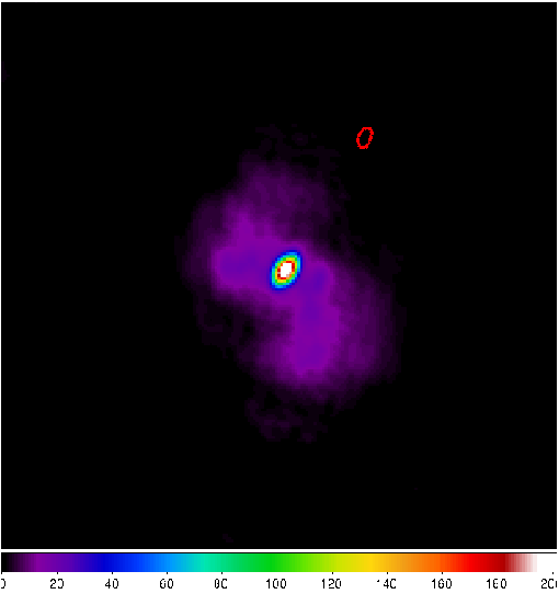
Fig. 35 Simulated image of Virgo-A. The red ellipse is the PSF.¶

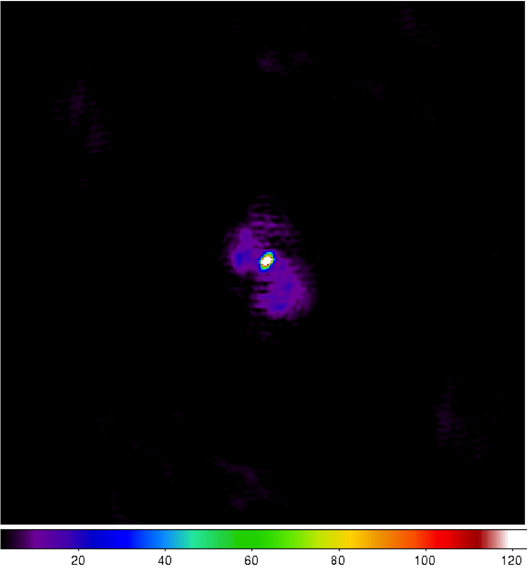
Fig. 36 Calibrated image of Virgo-A (uniform weights).¶

By looking at Fig. 35, we do not see any major discrepancy in our sky model (although we have lower resolution) so we go ahead with calibration.

Calibration¶

You can use the normal calibration procedure you adopt with any other LOFAR observation here. So we will not go into details. We have shown the image made after calibration in Fig. 36.

NOTE: It is advised to use uniform weights to compare the calibrated image to the model image.

Using Fig. 36, we can repeat our sky model construction to get a better result. This of course depends on your science requirements.

Residual¶

A better way to check the accuracy of your sky model is to subtract this model from the calibrated data and make an image of the residual. In Fig. 37, we have shown the residual for two subbands of 1.5 hour duration at 55 MHz. We clearly see an off center source (about 2 Jy) on top right hand corner.

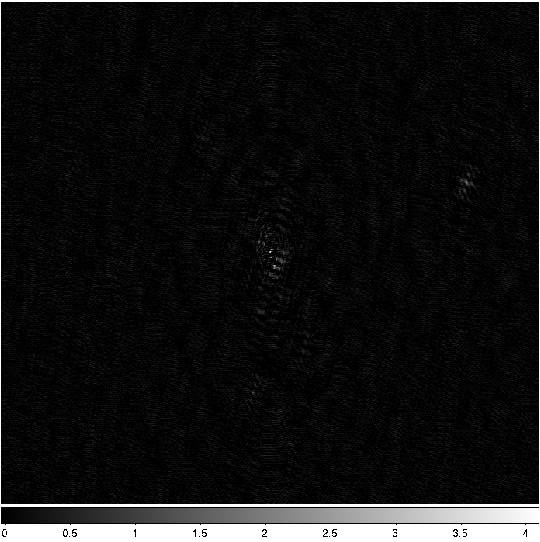
Fig. 37 Residual image of Virgo-A. An off center source is present on top right hand corner.¶

Recalibration¶

Once you have the residual image, you can also include to off center sources and update the sky model to re-calibrate the data.

Conclusions¶

We have given only a brief overview of the software and techniques in extended source modeling using shapelets. There are many points that we have not covered in this tutorial. However, we hope you (the user) will experiment and explore all available possibilities. Questions/Comments/Bug reports can be sent to Sarod Yatawatta.

References¶

S. Yatawatta, “Fundamental limitations of pixel based image deconvolution in radio astronomy,” in proc. IEEE Sensor Array and Multichannel Signal Processing Workshop (SAM), Jerusalem, Israel, pp. 69–72, 2010.
S. Yatawatta, “Radio astronomical image deconvolution using prolate spheroidal wave functions,” IEEE International Conference on Image Processing (ICIP) 2011, Brussels, Belgium, Sep. 2011.
1. Yatawatta, “Shapelets and Related Techniques in Radio-Astronomical Imaging,” URSI GA, Istanbul, Turkey, Aug. 2011.

Footnotes

1: The author of this chapter is Sarod Yatawatta.

Sky Model Construction Using Shapelets 1¶