LoSoTo: LOFAR Solution Tool 1

The LOFAR Solution Tool is a Python package which handles LOFAR solutions in a variety of ways. The data files used by LoSoTo are not in the standard parmdb format used by BBS/NDPPP (e.g. the “instrument” table). LoSoTo uses instead an innovative data file, called H5parm, which is based on the HDF5 standard.

LoSoTo can be accessed on CEP3 by

module load losoto

H5parm

H5parm is simply a list of rules which specify how data are stored inside the tables of an HDF5 compliant file. We can say that H5parm relates to HDF5 in the same way that parmdb relates to MeasurementSet. The major advantage of using HDF5 is that it is an opensource project developed by a large community of people. It has therefore a very easy-to-use Python interface (the pytables module) and it has better performance than competitors.

HDF5 format

There are three different types of nodes used in H5parm:

• Array: all elements are of the same type.

• CArray: like Arrays, but here the data are stored in chunks, which allows easy access to slices of huge arrays, without loading all data in memory. These arrays can be much larger than the physically available memory, as long as there is enough disk space.

• Tables: each row has the same fields/columns, but the type of the columns can be different within each other. It is a database-like structure.

The use of tables to create a database-like structure was investigated and found to be not satisfactory in terms of performance. Therefore LoSoTo is now based on CArrays organized in a hierarchical fashion which provides enough flexibility but preserves performance.

Characteristics of the H5parm

H5parm is organized in a hierarchical way, where solutions of multiple datasets can be stored in the same H5parm (e.g. the calibrator and the target field solutions of the same observation) into different solution-sets (solset). Each solset can be thought as a container for a logically related group of solutions. Although its definition is arbitrary, usually there is one solset for each beam and for each scan. Each solset can have a custom name or by default it is called sol### (where ### is an increasing integer starting from 000).

Each solset contains an arbitrary number of solution-tables (soltab) plus a couple of Tables with some information on antenna locations and pointing directions. Soltabs also can have an arbitrary name. If no name is provided, then it is by default set to the solution-type name (amplitudes, phases, clock, tec…) plus again an increasing integer (e.g. amplitudes000, phase000…). Since soltab names are arbitrary the proper solution-type is stated in the parmdb_type attribute of the soltab node. Supported values are: amplitude, phase, scalarphase, rotation, clock, tec, tecscreen and phase_offset.

Soltabs are also just containers; inside each soltab there are several CArrays which are the real data holders. Typically there are a number of 1-dimensional CArrays storing the axes values (see Table 2) and two $n$-dimensional (where \(n\) is the number of axes) CArrays, “values” and “weights”, which contain the solution values and the relative weights.

Soltabs can have an arbitrary number of axes of whatever type. Here we list some examples:

• amplitudes: time, freq, pol, dir, ant

• phases: time, freq, pol, dir, ant

• clock: time, ant, [pol]

• tec: time, ant, dir, [pol]

• foobar: foo, bar…

Theoretically the values/weights arrays can be only partially populated, leaving NaNs (with 0 weight) in the gaps. This allows to have e.g. different time resolution in the core stations and in the remote stations (obviously this ends up in an increment of the data size). Moreover, solution intervals do not have to be equally spaced along any axis (e.g. when one has solutions on frequencies that are not uniformly distributed across the band). The attribute axes of the “values” CArrays states the axes names and, more important, their order.

Table 2 Default names and formats for axes values.

Axis name	Format	Example
time (s)	float64	[4.867e+09, 4.868e+09, 4.869e+09]
freq (Hz)	float64	[120e6,122e6,130e6…]
ant	string	[CS001LBA]
pol	string (2 char)	[?XX?, ?XY?, ?RR?, ?RL?]
dir	string (16 char)	[?3C196?,?pointing?]
val	float64	[34.543,5345.423,123.3213]
weight (0 = flagged)	float32 [from 0 or 1]	[0,1,0.9,0.7,1,0]

Example of H5parm content

Here is an example of the content of an H5parm file having a single solset (sol000) containing a single soltab (amplitude000).

# this is the solset
/sol000 (Group) ''

# this is the antenna Table
/sol000/antenna (Table(36,), shuffle, lzo(5)) 'Antenna names and positions'
 description := {
 "name": StringCol(itemsize=16, shape=(), dflt='', pos=0),
 "position": Float32Col(shape=(3,), dflt=0.0, pos=1)}
 byteorder := 'little'
 chunkshape := (2340,)

# this is the source Table
/sol000/source (Table(1,), shuffle, lzo(5)) 'Source names and directions'
 description := {
 "name": StringCol(itemsize=16, shape=(), dflt='', pos=0),
 "dir": Float32Col(shape=(2,), dflt=0.0, pos=1)}
 byteorder := 'little'
 chunkshape := (2730,)

# this is the soltab
/sol000/amplitude000 (Group) 'amplitude'

# this is the antenna axis, with all antenna names
/sol000/amplitude000/ant (CArray(36,), shuffle, lzo(5)) ''
 atom := StringAtom(itemsize=8, shape=(), dflt='')
 maindim := 0
 flavor := 'numpy'
 byteorder := 'irrelevant'
 chunkshape := (36,)

# direction axis, with all directions
/sol000/amplitude000/dir (CArray(2,), shuffle, lzo(5)) ''
 atom := StringAtom(itemsize=8, shape=(), dflt='')
 maindim := 0
 flavor := 'numpy'
 byteorder := 'irrelevant'
 chunkshape := (2,)

# frequency axis, with all the frequency values
/sol000/amplitude000/freq (CArray(5,), shuffle, lzo(5)) ''
 atom := Float64Atom(shape=(), dflt=0.0)
 maindim := 0
 flavor := 'numpy'
 byteorder := 'little'
 chunkshape := (5,)

# polarization axis
/sol000/amplitude000/pol (CArray(2,), shuffle, lzo(5)) ''
 atom := StringAtom(itemsize=2, shape=(), dflt='')
 maindim := 0
 flavor := 'numpy'
 byteorder := 'irrelevant'
 chunkshape := (2,)

# time axis
/sol000/amplitude000/time (CArray(4314,), shuffle, lzo(5)) ''
 atom := Float64Atom(shape=(), dflt=0.0)
 maindim := 0
 flavor := 'numpy'
 byteorder := 'little'
 chunkshape := (4314,)

# this is the CArray with the solutions, note that its shape is the product of all axes
shapes /sol000/amplitude000/val (CArray(2, 2, 36, 5, 4314), shuffle, lzo(5)) ''
 atom := Float64Atom(shape=(), dflt=0.0)
 maindim := 0
 flavor := 'numpy'
 byteorder := 'little'
 chunkshape := (1, 1, 10, 2, 1079)

# weight CArray, same shape of the "val" array
/sol000/amplitude000/weight (CArray(2, 2, 36, 5, 4314), shuffle, lzo(5)) ''
 atom := Float64Atom(shape=(), dflt=0.0)
 maindim := 0
 flavor := 'numpy'
 byteorder := 'little'
 chunkshape := (1, 1, 10, 2, 1079)

H5parm benchmarks

For a typical single-SB parmdb of 37 MB the relative H5parm is around 5 MB large. A typical H5parm for an 8 hrs observation using 244 SBs is \(\sim 3\) GB (LBA) and \(\sim 5\) GB (HBA). Reading times between compressed and non-compressed H5parms are comparable within a factor of 2 (compressed is slower). Compared to parmdb the reading time of the python implementation of H5parm (mid-compression) is a factor of a few (2 to 10) faster.

This is a benchmark example:

INFO: H5parm filename = L99289-cal_SB081.h5
INFO: parmdb filename = L99289-cal_SB081.MS/instrument/
INFO: ### Read all frequencies for a pol/dir/station
INFO: PARMDB -- 1.9 s.
INFO: H5parm -- 0.28 s.
INFO: ### Read all times for a pol/dir/station
INFO: PARMDB -- 1.85 s.
INFO: H5parm -- 0.28 s.
INFO: ### Read all rotations for 1 station (slice in time)
INFO: PARMDB -- 1.94 s.
INFO: H5parm -- 0.3 s.
INFO: ### Read all rotations for all station (slice in time)
INFO: PARMDB -- 8.05 s.
INFO: H5parm -- 0.26 s.
INFO: ### Read all rotations for remote stations (slice in ant)
INFO: PARMDB -- 3.81 s.
INFO: H5parm -- 1.65 s.
INFO: ### Read all rotations for a dir/station and write them back
INFO: PARMDB -- 2.01 s.
INFO: H5parm -- 0.47 s.
INFO: ### Read and tabulate the whole file
INFO: parmdb -- 0.67 s.
INFO: H5parm -- 0.02 s.

LoSoTo

LoSoTo is made by several components. It has some tools used mostly to transform parmdb to H5parm and back (see the section on tools). A separate program (losoto.py) is instead used to perform operations on the specified H5parm. The script losoto.py receives its commands by reading a parset file that has the same syntax of BBS/NDPPP parsets (see losoto parset).

Tools

There are currently four tools shipped with LoSoTo:

• parmdb_benchmark.py provides a comparison between parmdb and H5parm for reading/writing

• parmdb_collector.py fetches parmdb tables from the cluster using a gds file

• H5parm_importer.py creates an h5parm file from an instrument table (parmdb) or a globaldb created by hand or with parmdb_collector.py

• H5parm_merge.py copies a solset from an H5parm files into another one

• H5parm_exporter.py exports an H5parm to a pre-existing parmdb

Details on how to use these tools are described below under section Usage.

Operations

These are the operations that LoSoTo can perform:

• ABS: takes the absolute value of the solutions (probably most meaningful for amplitudes).

• CLIP: clip all solutions $n$ times above and \(1/n\) times below the median value (only for amplitudes).

• CLOCKTEC: perform clock/tec separation (code maintained by Maaijke Mevius).

• DUPLICATE: duplicate a solution table.

• FARADAY: extract Faraday rotation solutions from the difference between RR and LL phase solutions.

• FLAG: iteratively remove a general trend from the solutions and then perform noisy region detection and outlier rejection. For phases this is done in real/imaginary space, for amplitude in log space.

• FLAGEXTEND: flag a point if surrounded by enough other flags in a chosen N-dimensional space

• INTERP: interpolate solutions along whatever (even multiple) axis. Typically one can interpolate in time and/or frequency. This operation can also simply rescale the solutions to match the median of the calibrator solution on a specific axis.

• NORM: normalize solutions of an axis to have a chosen average value.

• PLOT: plot solutions in 1D/2D plots.

• PLOTTECSCREEN: plot TEC screen (code maintained by David Rafferty).

• RESET: reset the solution values to 1 for all kind of solutions but for phases which are set to 0.

• RESIDUAL: subtract a table from another (e.g. remove TEC from phases).

• REWEIGHT: manually set weights to a specific values (can be used to hand-flag data, e.g. a bad antenna/timerange).

• SMOOTH: smooth solutions using a multidimensional running median. The n-dimensional surface generated by multiple axis (e.g. time and freq) can be smoothed in one operation using a different FWHM for each axis.

• TECFIT: fit TEC values per direction and station to phase solutions (code maintained by David Rafferty).

• TECSCREEN: fit TEC screens to TEC values (code maintained by David Rafferty).

• EXAMPLE: this is just an example operation aimed to help developing of new operations.

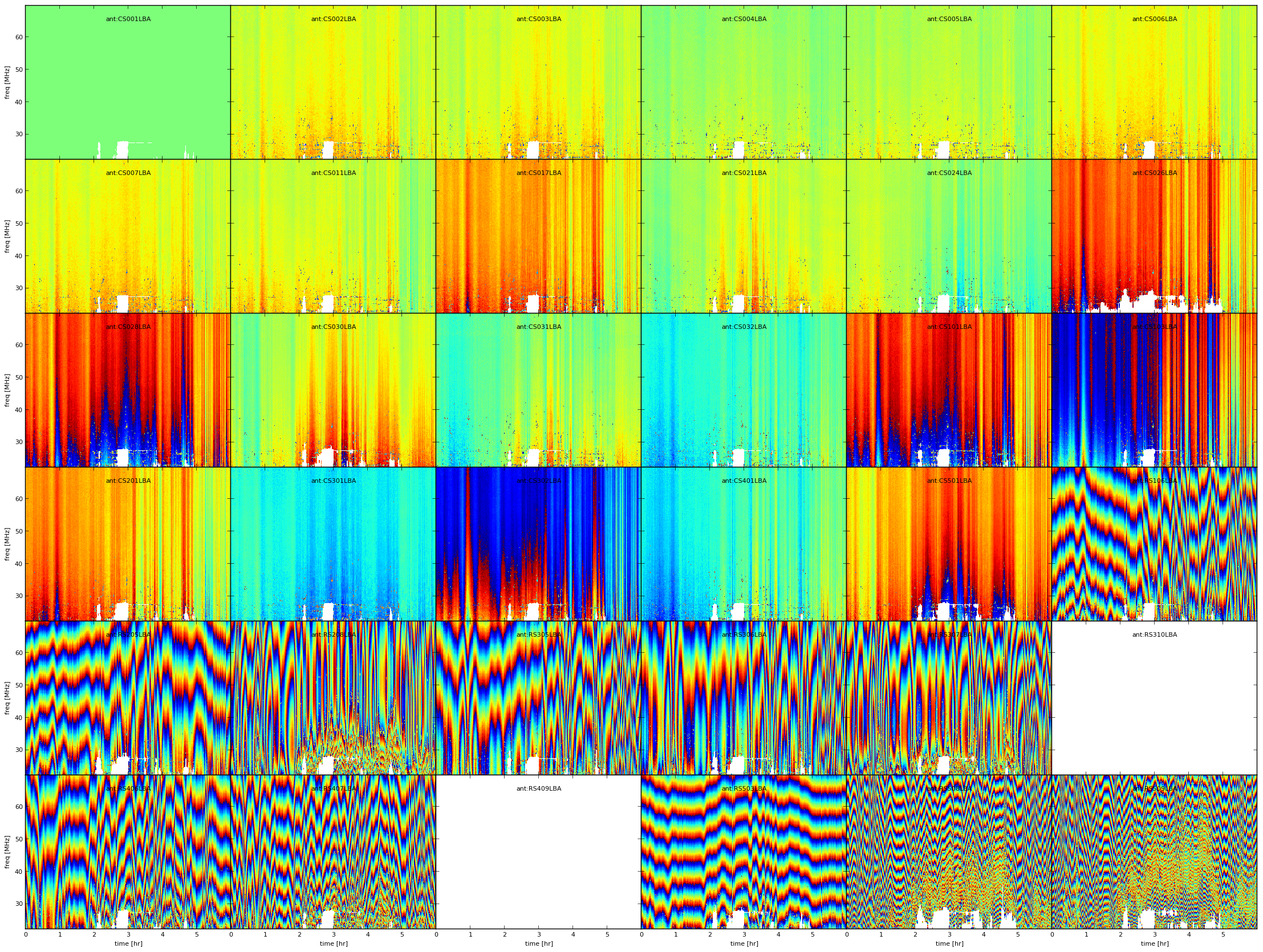
Fig. 6 Example phase solutions plotted using PLOT operation after the FLAG operation. White pixels are flagged data, every plot is an antenna, X-axis is time and Y-axis is frequency.

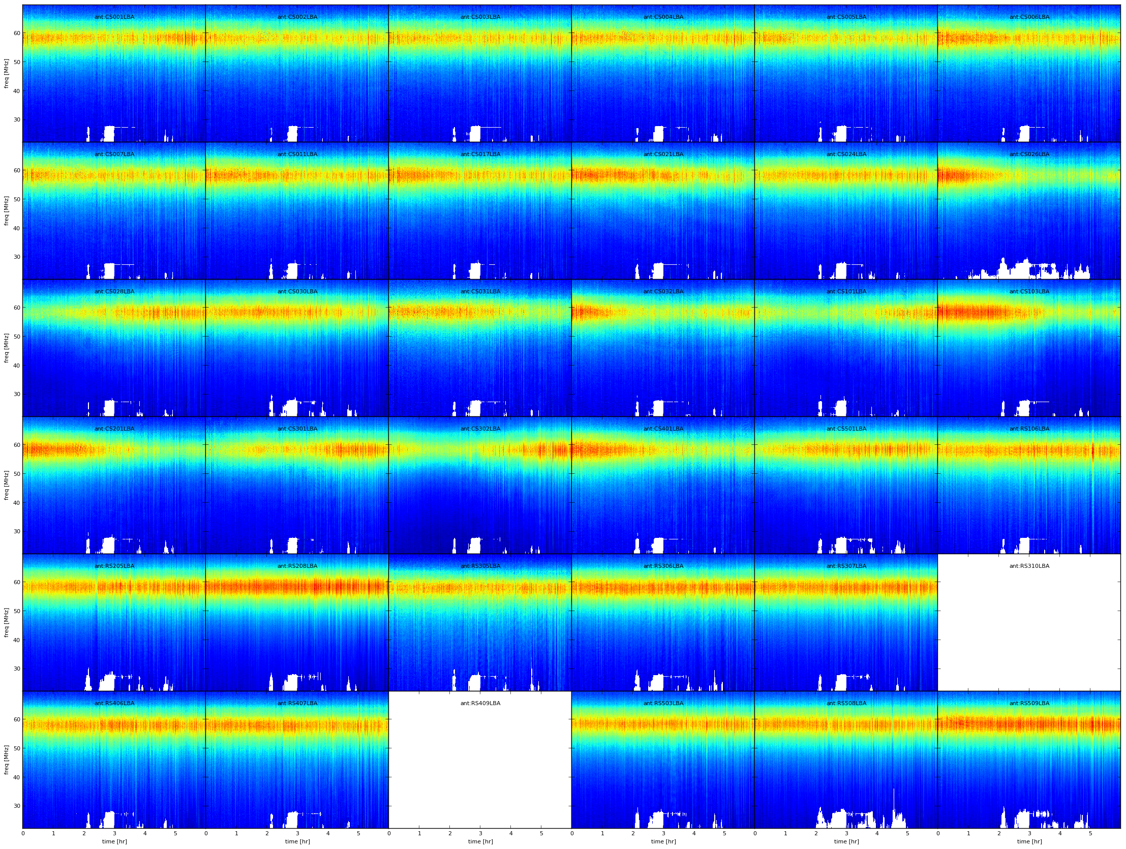
Fig. 7 Example amplitude solutions plotted using PLOT operation after the FLAG operation. White pixels are flagged data, every plot is an antenna, X-axis is time and Y-axis is frequency.

Beside these operations which require the activation through a LoSoTo parset file, one can call losoto.py with the “-i” option passing an H5parm as argument to obtain some information on it. Information on a specific subset of solsets can be obtained with “-i -f solset_name(s)”. If “-i” is combined with “-v” (verbose), LoSoTo will take a bit more time and outputs also the percentage of flagged data and the values of all axes will be written in a file (e.g. file.h5-axes_values.txt). Using the “-d” options instead one can delete a chosen soltab (e.g. “losoto.py -d sol000/phase000 file.h5”).

$ losoto.py -i -v single.h5
WARNING: Axes values saved in single.h5-axes_values.txt

Summary of single.h5

Solution set 'sol000':
======================

Directions: 3C196
            pointing

Stations: CS001LBA   CS002LBA   CS003LBA   CS004LBA
          CS005LBA   CS006LBA   CS007LBA   CS011LBA
          CS017LBA   CS021LBA   CS024LBA   CS026LBA
          CS028LBA   CS030LBA   CS031LBA   CS032LBA
          CS101LBA   CS103LBA   CS201LBA   CS301LBA
          CS302LBA   CS401LBA   CS501LBA   RS106LBA
          RS205LBA   RS208LBA   RS305LBA   RS306LBA
          RS307LBA   RS310LBA   RS406LBA   RS407LBA
          RS409LBA   RS503LBA   RS508LBA   RS509LBA

Solution table 'amplitude000' (type: amplitude): 2 pols, 2 dirs, 36 ants, 5 freqs,
4314 times
Flagged data 1.131%

   History:
   2014-12-17 13:29:25: CREATE (by H5parm_importer.py from
                        lof011:/home/fdg/scripts/losoto/examples/single.globaldb)

Solution table 'rotation000' (type: rotation): 2 dirs, 36 ants, 5 freqs, 4314 times
Flagged data 1.131%

   History:
   2014-12-17 13:29:25: CREATE (by H5parm_importer.py from
                        lof011:/home/fdg/scripts/losoto/examples/single.globaldb)

Solution table 'phase000' (type: phase): 2 pols, 2 dirs, 36 ants, 5 freqs, 4314 times
Flagged data 1.131%

   History:
   2014-12-17 13:29:25: CREATE (by H5parm_importer.py from
                        lof011:/home/fdg/scripts/losoto/examples/single.globaldb)

LoSoTo parset

This is an example parset for the interpolation in amplitude:

LoSoTo.Steps = [interp]
LoSoTo.Solset = [sol000]
LoSoTo.Soltab = [sol000/amplitude000]
LoSoTo.SolType = [amplitude]
LoSoTo.ant = []
LoSoTo.pol = [XX,YY]
LoSoTo.dir = []

LoSoTo.Steps.interp.Operation = INTERP
LoSoTo.Steps.interp.InterpAxes = [freq, time]
LoSoTo.Steps.interp.InterpMethod = nearest
LoSoTo.Steps.interp.MedAxes = []
LoSoTo.Steps.interp.Rescale = F
LoSoTo.Steps.interp.CalSoltab = cal000/amplitude000
LoSoTo.Steps.interp.CalDir = 3C295

In the first part of the parset “global” values are defined. These are values named LoSoTo.val_name. In Table 3, the reader can find all the possible global values.

Table 3 Definition of global variables in LoSoTo parset.

Variable name	Format	Example	Comment
LoSoTo.Steps	list of steps	[flag, plot, smoothPhases, plot2]	sequence of steps names in order
LoSoTo.Solset	list of solset names	[sol000, sol001]	restrict to these solsets
LoSoTo.Soltab	list of soltabs: Solset/soltab	[sol000/amplitude000]	restrict to these soltabs
LoSoTo.SolType	list of solution types	[phase]	restrict to soltab of this solution type
LoSoTo.ant	antenna names	[CS001_HBA]	restrict to these antenna
LoSoTo.pol	polarization	[XX, YY]	restrict to these polarizations
LoSoTo.dir 3	directions	[pointing, 3C196]	restrict to these pointing directions
LoSoTo.freq	frequencies	[30076599.12109375]	restrict to these frequencies
LoSoTo.time	times	[123456789.1234]	restrict to these times
LoSoTo.Ncpu 4	integer	10	number of processes of spawn

For every stepname mentioned in the global “steps” variable the user can specify step-specific parameters using the syntax: LoSoTo.Steps.stepname.val_name. At least one of these options must always be present, which is the “Operation” option that specifies which kind of operation is performed by that step among those listed under section Operations. All the global variables (except from the “steps” one) are also usable inside a step to change (override) the selection criteria for that specific step. Selection can be a string (interpreted as a regular expression), a list of values (exact match) or can have a min/max/step value which is activated using the axisName.minmax sintax (e.g. LoSoTo.freq.minmax = [30e6,1e9,5] to select 1 point every 5 from 30 MHz to 1 GHz). A list of step-specific parameters is given in https://github.com/revoltek/losoto.

Usage

This following is a possible sequence of commands to run LoSoTo on a typical observation:

• Collect the parmdb of calibrator and target:

  parmdb_collector.py -v -d "target.gds" -c "clusterdesc" -g globaldb_tgt
  parmdb_collector.py -v -d "calibrator.gds" -c "clusterdesc" -g globaldb_cal
  

where “[target/calibrator].gds” is the gds file (made with combinevds) of all the SB you want to use. You need to run the collector once for the calibrator and once for the target. “Clusterdesc” is a cluster description file as the one used for BBS (not stand-alone).

One can create the globaldb also by hand. Just create a directory, copy all the instrument (parmdb) tables you need calling them: instrument-1, instrument-2, and so on. Then copy from one of the MS (they are all the same) the ANTENNA, FIELD and sky tables. This directory is now a valid globaldb.

• Convert the set of parmdbs into an h5parm

  H5parm_importer.py -v tgt.h5 globaldb_tgt
  H5parm_importer.py -v cal.h5 globaldb_cal
  

This command converts ALL the instrument tables (parmdb) inside the globaldb directories in a single solset inside tgt.h5.

One can then merge the two h5parms in a single file (this is needed if you want to interpolate/rescale/copy solutions in time/freq from the cal to the target):

H5parm_merge.py -v cal.h5:sol000 tgt.h5:cal000

An easier approach is to directly append the second globaldb to the h5parm file of the first (note the same name for the h5parm)

H5parm_importer.py -v tgt.h5 globaldb_tgt
H5parm_importer.py -v tgt.h5 globaldb_cal

One can create a h5parm also from a single SB

H5parm_importer.py -v LXXXXX_3c295.h5 LXXXXX_3c295.MS

This command converts the “instrument” (parmdb) table inside the MS in a solset inside LXXXXX_3c295.h5. Note that given the definition of globaldb above, a single-SB measurement set is a perfect valid one.

• Run LoSoTo using e.g. the parset explained in LoSoTo parset

  losoto.py -v tgt.h5 losoto-interp.parset
  

• Convert back the h5parm into parmdb:

  H5parm_exporter.py -v -c tgt.h5 globaldb_tgt
  

• Redistribute back the parmdb tables into globaldb_tgt that are now updated (inspect with parmdbplot), there’s no automatic tool for that yet.

Developing in LoSoTo

LoSoTo is much more than a stand alone program, the user can use LoSoTo to play easily with solutions and to experiment. The code is freely available and is already the result of the collaborative effort of several people. If interested in developing your own operation, please have a look at: https://github.com/revoltek/losoto/.

In the “tools” directory the user can find all the tools described in section Tools plus some other program. All these programs are stand-alone. losoto.py is the main program which calls all the operations (one per file) present in the “operation” directory. It relays on the h5parm.py library which deals with reading and writing from an H5parm file and the operations_lib.py library which has some functions common to several operations.

An example operation one can use to start coding its own, is present in the “operation” directory under the name example.py. That is the first point to start when interested in writing a new operation. The most important thing shown in the example operation is the use of the H5parm library to quickly fetch an write back solutions in the H5parm file.

Clock/TEC separation

In LoSoTo an algorithm is implemented with which it is possible to separate the BBS phase solutions into a instrumental delay (clock) and an ionospheric component (TEC, a measure of the differential ionospheric electron content). This is done using the difference in frequency dependence of both effects: The phase shift due to a delay error goes as \(\nu\), whereas ionospheric refraction gives to first order an phase shift proportional to \(1/\nu\). Accordingly, one needs to have solutions over a large enough bandwidth to be able to do the separation 2.

There are three situations for which Clock/TEC separation could be useful. The first is if one needs to transfer from a calibrator not only the amplitudes, but also the phase solutions, eg. to be able to combine more sub-bands before doing a phase self-calibration on the target field. Since the ionospheric refraction is a direction dependent effect, in most cases it does not make sense to transfer the ionospheric phases. It is then possible to only apply the clock solutions from the calibrator to the target field. However, one should take note that the delays between stations drift and therefore this method is only useful if calibrator data was taken simultaneously with the target field.

A more experimental case for Clock/TEC separation is the fit of a TECscreen that can be applied during imaging with the AWimager, to correct for the direction dependent ionospheric effects. In this case, it is good to remove the direction independent instrumental effects as good as possible and only use the fitted TEC as input for the TECscreen. This has only been tested in very limited cases.

Finally, the TEC solutions of the clock/TEC separation give insight in the general ionospheric conditions of your observation. This could be of relevance if one wants eg. to estimate the noise due to remaining ionospheric errors.

It is important (especially for LBA) to correct for differential Faraday rotation before attempting to do a clock/TEC separation on the diagonal phases. The most straightforward way to do this, is to solve in BBS for diagonal gains and a common rotation angle.

The Clock/TEC fit as it is implemented in LoSoTo, returns per timeslot and station two arrays, one with clock errors (in s) and one with differential TEC solutions (in TEC-units). Furthermore a constant (in time) phase offset per station can be estimated. The remaining phase errors (eg. due to cable reflections) are of second order.

It is possible to write the clock solutions to the instrument tables and thus correct for them in BBS.

Footnotes

1

This chapter is maintained by Francesco de Gasperin.

2

The exact bandwidth requirements have not been tested yet, but it has been shown that on good S/N (calibrator) HBA data, it is possible to do the clock/TEC separation with 15 solutions, evenly distributed over 60 MHz.

3

It is important to notice that the default direction (e.g. those related to BBS solving for anything that is not “directional”:Gain, CommonRotationAngle, CommonScalarPhase, and so on) has the direction named “pointing”.

4

Only some operations have been parallelized.