Factor: Facet Calibration for LOFAR 1

Factor is a Python package that allows for the production of wide-field HBA LOFAR images using the facet calibration scheme described in van Weeren et al. (2016) to correct for direction-dependent effects (DDEs). To initialize your environment for Factor, users on CEP3 should run the following command:

source ~rafferty/init_factor

If you want to install Factor yourself, follow the instructions in the README.md file on the Factor GitHub repository. Detailed documentation for Factor can be found here.

Data preparation: Pre-facet calibration pipeline 2

The input data to Factor must have the average amplitude scale set and average clock offsets removed. Furthermore, the LOFAR beam towards the phase center should be removed. The data should be concatenated in frequency to bands of about 2 MHz bandwidth (so about 10–12~subbands). All bands (= input measurement sets) need to have the same number of frequency channelsfootnote{Factor does lots of averaging by different amounts to keep the data-size and computing time within limits. If the input files have different numbers of channels then finding valid averaging steps for all files gets problematic.}. Also the number of channels should have many divisors to make averaging to different scales easy. The data should then undergo direction-independent, phase-only self calibration, and the resulting solutions must be provided to Factor.

The pre-facet calibration pipelines are intended to prepare the observed data so that they can be used in Factor. The pipelines are defined as parsets for the genericpipeline, that first calibrate the calibrator, then transfer the gain amplitudes, clock delays and phase offsets to the target data, do a direction-independent phase calibration of the target, and finally image and subtract sources.

Please have a look at the documentation for the genericpipeline here. You should be reasonably familiar with setting up and running a genericpipeline before running this pipeline parset.

Download and set-up

The pipeline parsets and associated scripts can be found on the Prefactor GitHub repository. These pipelines require as input data that has been pre-processed by the ASTRON averaging pipeline. They can work both with observations that had a second beam on a calibrator and with interleaved observations in which the calibrator was observed just before and after the target. No demixing is done, but A-Team clipping is performed for the target data 3.

To run the genericpipeline you need a correctly set up configuration file for the genericpipeline. Instruction for setting up the configuration file can be found online. In addition to the usual settings you need to ensure that the plugin scripts are found, for that you need to add the pre-facet calibration directory to the recipe_directories in the pipeline parset (so that the plugins directory is a subdirectory of one of the recipe_directories).

Overview and examples

The most recent overview of the pre-facet pipeline functionality as well as several use cases and troubleshooting information can be found on the pre-facet pipeline GitHub wiki.

After the pipeline was run successfully, the resulting measurement sets are moved to the specified directory. The instrument table of the direction-independent, phase-only calibration are inside the measurement sets with the names instrument_directioninpendent. These measurement sets are the input to the Initial-Subtract pipeline, which should be run next to do the imaging and source subtraction. Once the Initial-Subtract pipeline has finished, the data are ready to be processed by Factor.

Factor tutorials

This section includes examples of setting up and using Factor. Setting up a Factor run mainly involves creating a parset that defines the reduction parameters. For many of these parameters, the default values will work well, and hence their values do not need to be explicitly specified in the parset. Therefore, only the parameters relevant to each example are described below. A detailed description of all parameters can be found on the online.

Quick-start

Below are the basic steps in a typical Factor run on a single machine (e.g., a single CEP3 node).

• Collect the input bands and Initial-Subtract sky models (produced as described in sub-section ref{factor:pre-facet-pipeline}) in a single directory. The MS names must end in “.MS” or “.ms”:

  [/data/factor_input]$ ls
  L99090_SB041_uv.dppp_122298A79t_119g.pre-cal.ms
  L99090_SB041_uv.dppp_122298A79t_119g.pre-cal.wsclean_low2-model.merge
  L99090_SB041_uv.dppp_122298A79t_121g.pre-cal.ms
  L99090_SB041_uv.dppp_122298A79t_121g.pre-cal.wsclean_low2-model.merge
  L99090_SB041_uv.dppp_122298A79t_123g.pre-cal.ms
  L99090_SB041_uv.dppp_122298A79t_123g.pre-cal.wsclean_low2-model.merge
  L99090_SB041_uv.dppp_122298A79t_125g.pre-cal.ms
  L99090_SB041_uv.dppp_122298A79t_125g.pre-cal.wsclean_low2-model.merge
  

• Edit the Factor parset (see online documentation for a detailed description) to fit your reduction and computing resources. For example, the parset for a single machine could be:

  [/data]$ more factor.parset
  [global]
  dir_working = /data/factor_output
  dir_ms = /data/factor_input
  
  [directions]
  flux_min_jy = 0.3
  size_max_arcmin = 1.0
  separation_max_arcmin = 9.0
  max_num = 40
  

• Run the reduction:

  [/data]$ runfactor factor.parset
  

Selecting the DDE calibrators and facets

Before facet calibration can be done, suitable DDE calibrators must be selected. Generally, a suitable calibrator is a bright, compact source (or a group of such sources) 4. The DDE calibrators can be provided to Factor in a file (see online documentation for details) or can be selected internally. This example shows how to set the parameters needed for internal selection.

Three parameters in the [directions] section of the parset are most important for the internal calibrator selection: flux_min_Jy, size_max_arcmin, and separation_max_arcmin. These parameters set the minimum flux density (in the highest-frequency band) and maximum size of the calibrators and the maximum allowed separation that two sources may have to be grouped together as a single calibrator (see online documentation for details). The following are good values to use as a starting point:

[directions]
flux_min_Jy = 0.3
size_max_arcmin = 1.0
separation_max_arcmin = 9.0

It is recommended that you set interactive = True under [global] while experimenting with the calibrator selection, as Factor will select the calibrators and then pause to allow you to verify them. Now, run Factor (with runfactor factor.parset) and once it asks for verification, open one of the *high2} images generated during the Initial Subtract pipeline in ds9 or casaviewer. Then load the region files located in the dir_working/regions/} directory (where dir_working is the working directory defined in your Factor parset). Fig. 14 shows an example of such an image with the regions overlaid.

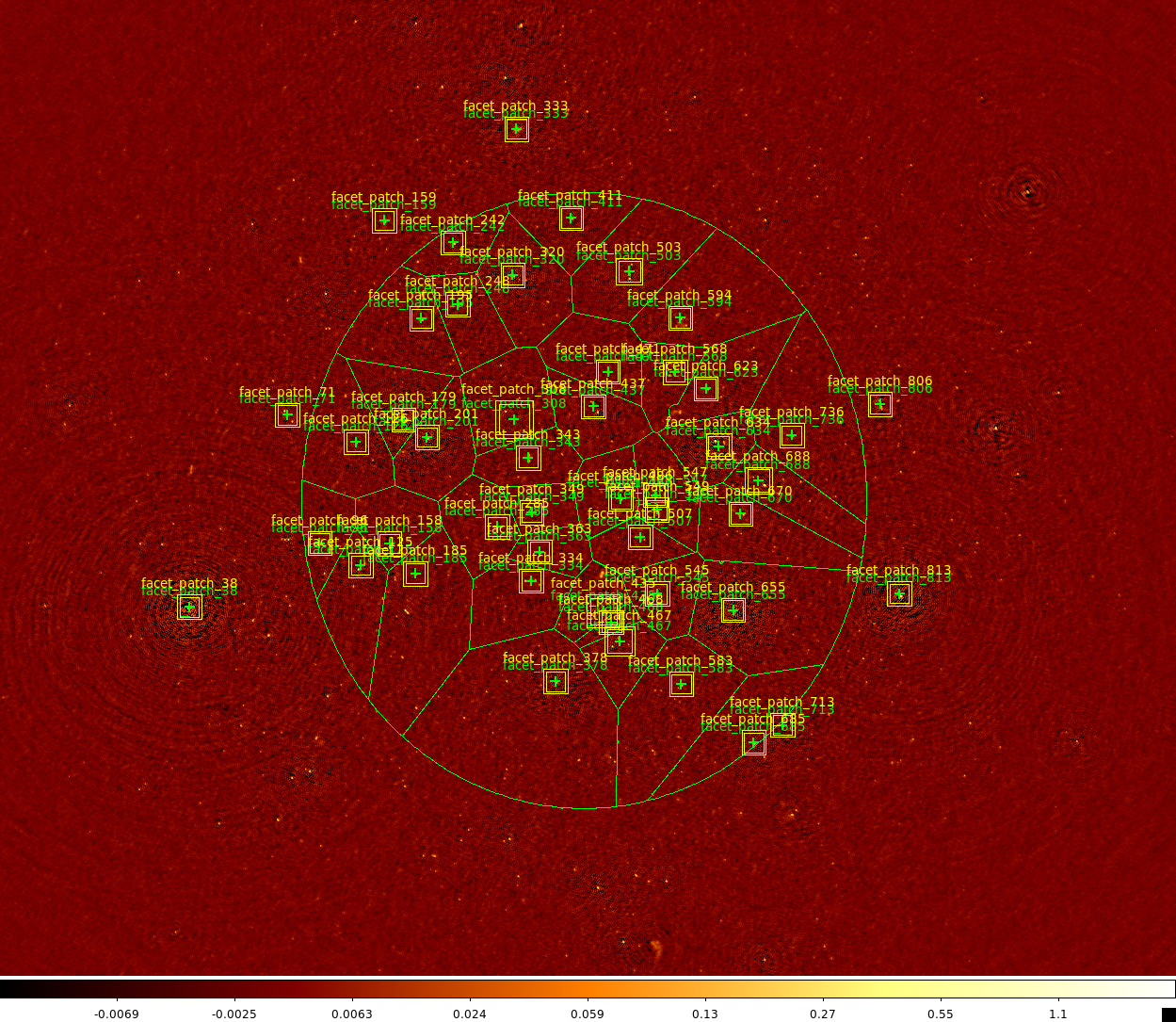
Fig. 14 Example of internally generated calibrators and facets. Yellow boxes show the regions to be imaged during self calibration (the inner box shows the region over which sources are added back to the empty datasets) and green regions show the facets. Each direction is labeled twice: once for the calibrator region and once for the facet region. Note the elliptical region that encompasses the faceted area. This region is controlled by the faceting_radius_deg parameter under [directions] in the parset: inside this radius (adjusted for the mean primary beam shape), full facets are used; outside this radius, only small patches are used that are much faster to process. This radius can be adjusted to limit the size of the outer facets and the region to be imaged.

Check that none of the calibrator image regions are overlapping significantly. If they are, try adjusting the above parameters to either group the calibrators together (so that they form a single calibrator) or remove one of them. Also check that no facet is larger than a degree or so. If such large facets are present, try adjusting the above parameters to obtain more calibrators (e.g., by lowering flux_min_Jy). If the large facets are on the outer edge of the faceted region, you should also consider reducing faceting_radius_deg to limit their size.

Once the calibrator and facet selection is acceptable, Factor will make a directions file named factor_directions.txt in dir_working. This file can now be edited by hand if desired (e.g., to specify a sky model or clean mask for a calibrator).

Imaging a target source

If you are interested only in a single target source, you may want to process just the brightest sources in the field and those nearest the target. Fig. 15 shows the layout of an example field, with the target source (a galaxy cluster) indicated by the blue circle in facet_patch_468. Note that the faceting radius has been reduced substantially to speed up processing (since facets outside of this radius are small patches that run much more quickly than full facets). A few facets (e.g., facet_patch_566 and facet_patch_273) contain bright sources with artifacts that affect the target. Additionally, although they contain fainter sources, artifacts from the neighboring facets (e.g., facet_patch_424) can also affect the target significantly. Therefore, a good strategy is to process these facets before processing the target. Note that the lowest possible noise would be obtained by processing the entire field but would require much longer to complete.

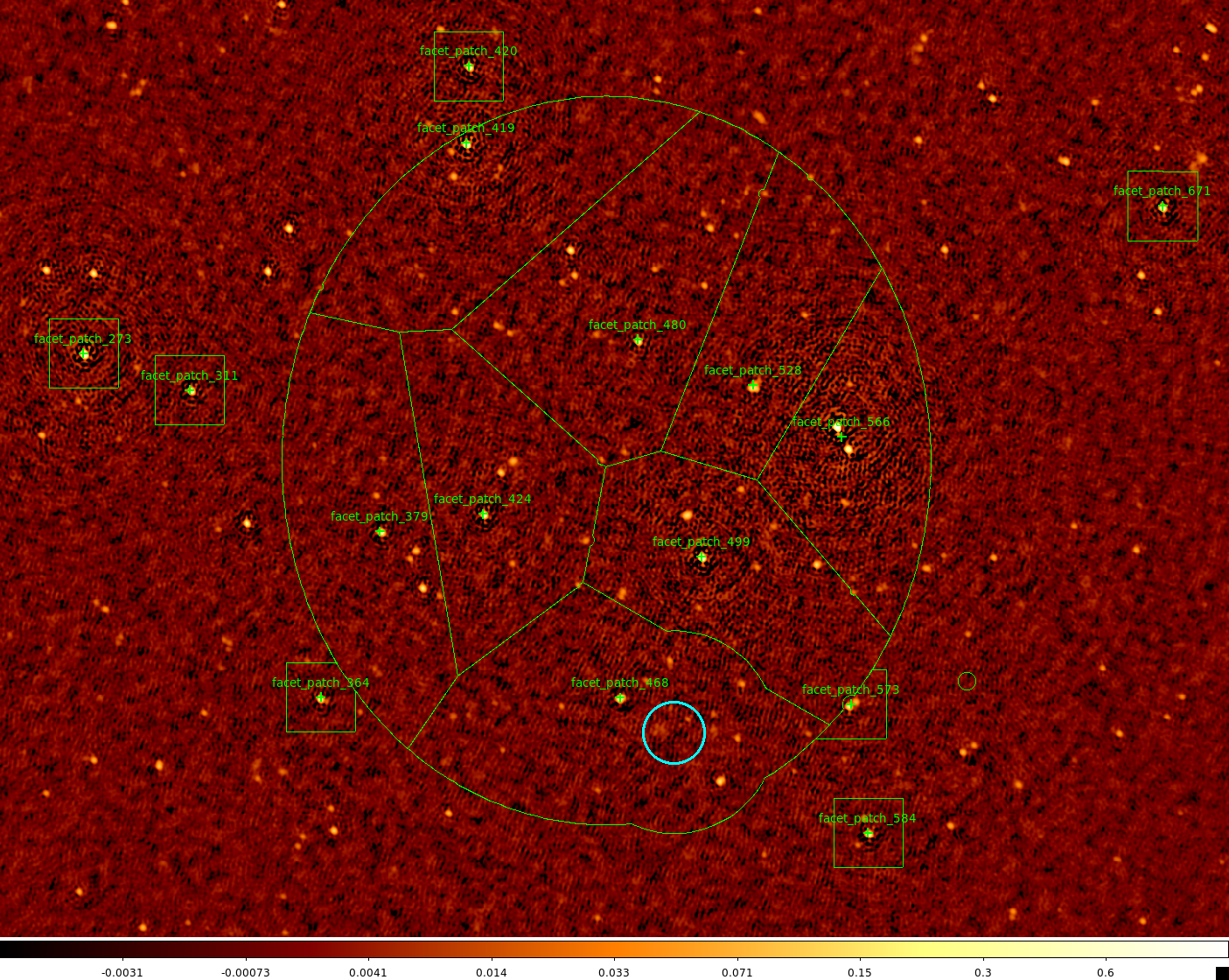
Fig. 15 Example of the field layout for a case in which an image is desired only for a single target source (indicated by the blue circle). A region of avoidance was also specified (with a larger radius than the blue circle) that resulted in the curved bulges to the boundary to the north and south of the target.

We can limit the processing to the sources above by moving them to the top of the directions file (named dir_working/factor_directions.txt if generated automatically) and setting ndir_process under [directions] in the parset to the number of sources we wish to be processed (including the facet with the target source). Note that you should typically have many more calibrators in the directions file than directions to be processed, as the facets shapes and sizes are determined from all calibrators together and too few can result in very large facets. An example directions file is shown below (note that only the first two columns are shown). In this case, the target facet (facet_patch_468) will be the seventh direction to be processed, so we set ndir_process = 7 under [directions] in the parset. Lastly, set image_target_only = True under [imaging] so that only the target facet is imaged.

# name position ...

facet_patch_566 14h29m38.5962s,44d59m14.0061s ...
facet_patch_499 14h31m36.5221s,44d41m39.6252s ...
facet_patch_424 14h34m38.5876s,44d48m00.415ss ...
facet_patch_379 14h36m04.2603s,44d45m16.2451s ...
facet_patch_273 14h40m14.6989s,45d10m53.6821s ...
facet_patch_573 14h29m33.1473s,44d19m43.2515s ...
facet_patch_468 14h32m44.3536s,44d20m50.7736s ...
......
facet_patch_550 14h30m03.9315s,46d51m44.6965s ...
facet_patch_480 14h32m28.9389s,45d13m49.3407s ...
facet_patch_778 14h20m03.7803s,44d09m40.3293s ...

Additionally, if the target source is diffuse, Factor may not be able to adjust the facet boundaries properly to ensure that it lies entirely within a single facet. To ensure that no facet boundary passes through the target source, you can define the position and the size of an avoidance region under the [directions] section of the parset. The target_ra, target_dec, and target_radius_arcmin parameters determine this avoidance region. An example of such a region for the target above is given below and the resulting facets are shown in Fig. 14. Note that the boundaries of the target facet (facet_patch_468) are curved to avoid this region.

[directions]
target_ra = 14h31m59.7s
target_dec = +44d15m48s
target_radius_arcmin = 15

Peeling bright sources

In many observations there will be one or more strong sources that lie far outside the FWHM of the primary beam but nevertheless cause significant artifacts inside it. However, because of strong variations in the beam with frequency at these locations, self calibration does not generally work well. Therefore, Factor includes the option to peel these outlier sources. A high-resolution sky model (in makesourcedb format) is needed for this peeling. Factor includes a number of such sky models for well-known calibrators (see online documentation for a list). If an appropriate sky model is not available inside Factor, you must obtain one and specify it in the directions file. To enable peeling, the outlier_source entry in the directions file must be set to True for the source.

It is also possible that a strong source (such as 3C295) will lie inside a facet. Such a source can be peeled to avoid dynamic-range limitations. Peeling will be done if a source exceeds peel_flux_Jy (set under the [calibration] section of the parset) and a sky model is available. After peeling, the facet is then imaged as normal.

Checking the results of a run

You can check the progress of a run with the checkfactor script by supplying the Factor parset as follows:

[/data]$ checkfactor factor.parset

A plot showing the field layout will be displayed (see Fig. 16), with facets colored by their status. Left-click on a facet to see a summary of its state, and press “c” to see a plot of the self calibration images and their clean masks. An example of such a plot is shown in Fig. 17. For a successful self calibration, you should see a gradual improvement from image02 to image42.

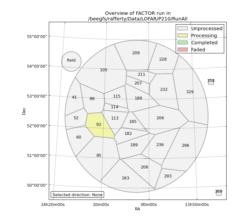
Fig. 16 Example checkfactor plot.

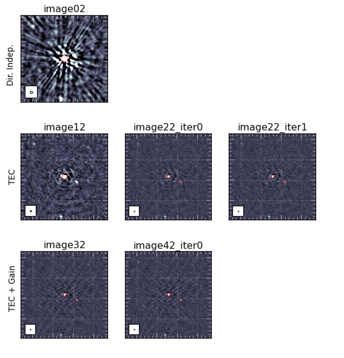
Fig. 17 Example of self calibration images for a successful run. The self calibration process starts with image02 (the image obtained after applying only the direction-independent solutions from pre-Factor) and proceeds to image12, image22, etc. In some cases, Factor will iterate a step until no more improvement is seen. These steps are indicated by the “iter” suffix.

If self calibration has completed for a direction, select it and press “t” to see plots of the differential TEC and scalar phase solutions and “g” to see plots of the slow gain solutions. These plots can be useful in identifying periods of bad data or other problems.

Dealing with failed self calibration

Self calibration may occasionally fail to converge for a direction, causing to Factor to skip the subtraction of the corresponding facet model. An example in which self calibration failed is shown in Fig. 18. Note how the image noise does not improve much in this case during the self calibration process. While Factor can continue with the processing of other directions and apply the calibration solutions from the nearest successful facet to the failed one (depending on the value of the exit_on_selfcal_failure option under [calibration] in the parset; see online documentation for details), it is generally better to stop Factor and try to correct the problem. In these cases, turning on multi-resolution self calibration or supplying a custom clean mask may improve the results.

Multi-resolution self calibration involves imaging at decreasing resolutions, from 20 arcsec to full resolution (\(\approx 5\) arcsec). This process can stabilize clean in the presence of calibration errors. An example of such a situation is shown in Fig. 18. Multi-resolution self calibration can be enabled by setting multires_selfcal = True under [calibration] in the parset.

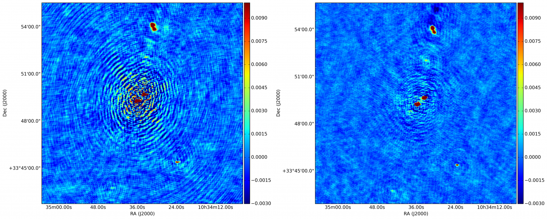
Fig. 18 Example of self calibration images at the same stage of reduction for an unsuccessful run (left) in which an incorrect source structure is present (the bright sources both have “L”-shaped morphologies) and the successful run (right) in which multi-resolution self calibration was used.

In some cases, usually when the calibrator has a complex structure, it may be necessary to supply a clean mask made by hand. Such a clean mask can be made by opening one of the self calibration images (e.g., *image22.image; see online documentation for details of the facetselfcal output) in casaviewer and drawing a region that encloses the source emission but excludes any artifacts. Save the region in CASA format to a file and specify the full path to this file in the region_selfcal column of the directions file (named dir_working/factor_directions.txt if generated automatically) for the appropriate direction. Note that the supplied mask must include all significant emission within the self calibration region.

Lastly, it is possible that the DDE calibrator is too faint to produce good self calibration results. In this case, the slow-gain solutions are generally noisy and the images produced after the slow-gain calibration (e.g., *image32.image) are worse than those before ((e.g., *image22.image). To fix this problem, either process other, brighter facets first (to lower the overall noise) or skip self calibration of the problematic facet.

To restart self calibration for the failed direction, you will need to reset it. See the section on resuming and resetting a run below for instructions on how to reset a direction.

Imaging at the end of a run

By default, once self calibration has been completed, Factor will image all facets at full resolution (1.5 arcsec cellsize, robust of -0.25, and no taper). To image the facets with different parameters, set one or more of the following facet parameters in the parset under [imaging]: facet_cellsize_arcsec, facet_robust, facet_taper_arcsec, and facet_min_uv_lambda. These parameters can be lists, with one set of images for each entry. For example, the following settings will make two images per facet, one at full resolution (1.5 arcsec cellsize, robust of -0.25, and no taper) and one at lower resolution (15 arcsec cellsize, robust of -0.5, and a 45 arcsec taper):

[imaging]
facet_cellsize_arcsec = [1.5, 15.0]
facet_robust = [-0.25, -0.5]
facet_taper_arcsec = [0.0, 45.0]

This run will produce two output directories: dir_working/results/facetimage/ (with the full-resolution images) and dir_working/results/facetimage_c15.0r-0.5t45.0u0.0/ (with the lower-resolution images).

Resuming and resetting a run

If a Factor run is interrupted, it can be resumed by simply running it again with the same command. Occasionally, however, you will want to change some settings (e.g., to supply a clean mask for self calibration) or something will go wrong that prevents resumption. In these cases, you can reset the processing for a direction with the “-r” flag to runfactor. For example, to reset direction facet_patch_350, the following command should be used:

runfactor factor.parset -r facet_patch_350

Finding the final output products

Usually, the final, primary-beam-corrected image of the field or target will be located in dir_working/results/fieldmosaic/field and will be called *correct_mosaic.pbcor.fits. A full description of the primary output products generated by Factor is available online.

Additionally, it may be desirable to image a facet by hand using the calibrated data (e.g., to ensure that any diffuse emission is properly cleaned). To do so, one can use archivefactor (see archiving a factor run) to archive the calibrated data for a facet in a convenient form for use in CASA or WSClean. Note that these data have not been corrected for any primary beam attenuation but have had the beam effects at the field phase center removed.

Archiving a Factor run

A Factor run can be archived at any point with archivefactor. For example, the following will produce a minimal archive (including images and plots, but no visibility data):

archivefactor factor.parset dir_output

To include the calibrated visibility data for one of more facets in the archive, add the “-d” flag followed by the names of the facets:

archivefactor factor.parset dir_output -d facet_patch_468,facet_patch_350

Lastly, to make an archive from which a Factor run can later be resumed, use the “-r” flag:

archivefactor factor.parset dir_output -r

To resume from such an archive, use unarchivefactor. See the online documentation for details.

Footnotes

1

This chapter is maintained by David Rafferty.

2

This section was written by Andreas Horneffer with a lot of help from Tim Shimwell.

3

Versions of the pipeline (parset) which also do demixing are being planned.

4

Ideally calibrators should be selected that provide roughly uniform coverage of the field with separations less than the typical distance over which the direction-dependent effects vary strongly (this distance depends on the severity of the ionospheric conditions, but is usually less than a degree or so). However, the achievable uniformity of coverage will vary from field to field, depending on the specific distribution of sources.