Data inspection 1 ¶

Data inspection is essential for a proper data reduction and can be carried out using either scripts (by means of a python interface to the Measurement Set) or CASA. In this Chapter, we summarize the various tools that can be used to inspect the LOFAR visibilities at the beginning and during the processing of your data.

The quality of raw measurement sets can be inspected using data quality inspection plots that are generated by the ASTRON staff. These plots are available online for up to three weeks after the time of observation. After that period, they are compressed and stored offline. Users can access them by creating a ticket through the JIRA Helpdesk.
The program msoverview provides you with details on the contents of a Measurement Set, no matter if it is raw or it has been already processed. You are advised to use this script when you start working on your data. You can run it by typing
```
msoverview in=some.MS verbose=T
```

where the verbose parameter allows you to have more detailed information about the observation, as the used antennas and their positions.

Python-casacore (formerly “pyrap”) is a python interface to the casacore library, which allows the raw data tables (Measurement Sets) to be manipulated and the data plotted via python scripts. These allow you to customize what is plotted, and can be significantly faster than CASA for plotting large datasets. An extensive description of the python-casacore utilities is available online.
Visibilities can be plotted relatively rapidly by making use of the combination of python-casacore and the plotting package PGPLOT, both of which work quickly. The script uvplot.py 2 can be used to plot visibility data and can be significantly faster than the PLOTMS task in CASA.
CASA is the python-based next generation replacement for AIPS and can be used to display the data.

Be aware that trying to inspect the raw visibilities with CASA will produce a “segmentation fault” error. To avoid this, you should make a copy of the dataset with DPPP (see the first example parset in Sect.~ref{theparsetfile}). Also note that the Radio Observatory now stores the LOFAR data as Dysco compressed measurement sets and hence CASA cannot be used to inspect them. You must decompress the measurement set first if you want to use CASA for data inspection 3. Moreover, when opening with CASA a MeasurementSet observed between May and October 2011, you will get an Unrecognized mount type error 4.

CASA has multiple functionalities that allows one to inspect different data products.

- casabrowser can be used to inspect the content of a Measurement Set.

- casaplotms can be used to visibility data against different parameters.

- casaviewer can be used to inspect images.

- For a detailed information and examples of how to use CASA, we direct users to the CASA Guides.
The low frequency radio sky is dominated by a few bright sources that form the so called A-team: CasA, CygA, VirA, TauA, HydA, HerA. The removal of these sources from the target visibilities is very important in order to achieve high dynamic range images. The script plot_Ateam_elevation.py, which is available as part of the LOFAR repository, can be used to inspect the contribution of these A-team sources to the observed visibility data.
For manipulating measurement sets, you can use TaQL (Table Query Language); this is an SQL-like language which works on MS, and can perform all kinds of selections (and more). A detailed documentation of TaQL can be found here.

Analyzing the data quality with aoqplot¶

Once you have successfully run DPPP on the measurement sets in your observation, it is recommended that you validate the results of the flagger and get an impression of the quality of the full observation. For this, the aoqplot tool that is part of the LofIm build can be used.

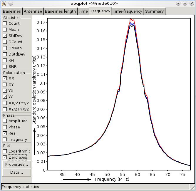
Basically, the tool allows you to plot standard deviations and RFI percentages and some other quantities, over time, frequency, baselines and the time-frequency domain of the full observation, i.e., over all sub-bands. Since an observation can be several terabytes of data, the performance of standard tools to perform such analysis is an issue, and the aoqplot was designed to overcome this problem. Fig.~ref{aoqplot-window} shows an example of the aoqplot interface, plotting the data standard deviations of an LBA set over the entire frequency range. It also allows one to plot differential statistics. “Differential” in this context means that the standard deviation is calculated over the difference between adjacent channels. Therefore, they quantify the noise, because the difference of signal in adjacent (3 kHz) channels is tiny and can be neglected. Differential quantities are prefixed with a “D”, such as DMean and DStdDev.

Fig. 1 The aoqplot window showing the standard deviation of the data over frequency of a full observation.¶

Usage¶

If your environment allows (see below), one can get the statistic plots of an observation of a DPPPed set, with the following command:

$ aoqplot yourobservation.gvds

The gvds file is given by the observatory and describes the observation, in particular the locations of the measurement sets. The aoqplot tool will now connect to all the nodes with an ssh connection, start a bash-session on the node and start a client there that connects back to your node and sends the quality tables. Once all the tables have been received, a window will appear containing the plots. Collecting all the tables takes typically less than 5 seconds.

The use of ssh and bash requires that you should be able to ssh to all the involved nodes without manual intervention, and that the client (called aoremoteclient, part of the LofIm daily build) is directly in your bash path after ssh-ing. Thus, after ssh lof001, you should be able to start aoremoteclient within bash without a module load lofar. The easiest way of doing this is by putting lofar in $HOME/.mypackages. If you have problems running the aoqplot due to your environment, please let us know.

When a node is not answering, or there is some error with the measurement set, the set will be skipped, an error will be given describing the problem and the statistics will be collected without those measurement sets. If none of the measurement sets can be queried, you will see a dialog window with many error messages and the window will not appear thereafter. If you can not determine the cause of this, please let us know. The software is currently (January 2012) still experimental.

The aoqplot can also be used on individual sub-bands by putting the measurement set filename in the command line, e.g.:

aoqplot SB000.MS

Analyzing the statistics¶

The aoqplot tool provides the following statistics:

Count: the number of samples that are left after flagging of the data. This should normally be fairly constant over time, frequency and baselines, apart from a few imprints of RFI that lower the number of available samples. Since the flags of the complex values of different polarizations are normally equal, there’s no use in looking at this statistic for polarizations or real/imaginary components indivually.
Mean: the mean of the data. If you are observing a strong source (such as a calibrator), this value should contain structure over time, frequency and baselines. Note that if you for example plot the mean over time, each sample in the plot shows the mean of that timestep over all baselines and frequencies. Therefore, if your source is not in the phase centre, it will be supressed and can even be averaged out, because sources outside the phase centre contribute sinusoidally and will cancel out. If your source is in the phase centre, the Mean is a very good representation of the strength of the signal. Together with an estimate of the noise, this can be used to calculate the signal-to-noise ratio during the observation. If you know the approximate flux density of the source, you can estimate the gain during the observation and, together with an estimate of the noise, calculate a rough estimate of the system noise. Cross polarizations can be checked to see if there was significant differential Faraday rotation during the observation.
StdDev: the standard deviation of the data after flagging. The standard deviation should not have significant imprints of RFI. In good data, one generally sees about three significant spikes in HBA (in $\pm$ 115-163 MHz) and zero spikes in LBA (>30 MHz, an example is given in Fig.~ref{aoqplot-window}). The standard deviation is rather sensitive for low-level RFI, and a few RFI spikes do not seem to hurt calibration at this point (please report if you think otherwise). If there are time or frequency ranges at which the standard deviation is significantly different, try to select different polarizations and use the different domains (time-frequency, baseline, time, frequency, …) to see if you can localize the guilty data range. The position of the Sun and the Milky Way in the sky can significantly change the standard deviation. Because the StdDev includes the variance of the signal, it is recommended also to look at the DStdDev.
DCount, DMean and DStdDev are similar to the above statistics, but are calculated over the differences of samples (after flagging) in adjacent channels. They contain therefore very little contribution of the signal, and can be used to get an accurate estimate of the noise. They have been normalized to represent the same units as their counterpart values. The DMean should be close to zero, as the signal should be subtracted out, and the noise should average out (it is mainly there because it is easy to calculate, but it is often more helpful to look at Mean and DStdDev).
RFI: the amount of RFI found by the flagger. The ‘base level’ of RFI is 2–5%, but can contain a few spikes over time or frequency that go up to 20%–100% at times. This is normally not a problem. Sub-bands or stations with significant different RFI levels (either 0% or $>\sim 5$%) often indicate an issue with the station. Such problems are often also reflected in the standard deviations. Different polarizations and real/imaginary values have equal RFI ratios.
SNR: the signal-to-noise ratio. It is calculated by Mean / DStdDev. This value is only accurate if you are observing a source in the phase centre, due to the reasons mentioned in the paragraph for the Mean value.

Background information¶

The aoqplot tool works together with DPPP. Recent versions (>21 December 2011) of DPPP will add so-called quality statistic tables to a measurement set. These tables circumvent having to read the entire DATA column of a measurement set to get the basic statistics. The way they are stored is described in the quality statistics proposal written by Andr'e Offringa. Because the statistics plotting tool require these tables, you can not directly plot statistics of measurement sets that are averaged by an older DPPP, or have not been averaged at all.

The statistics are calculated individually for the real and complex values. This is not common when treating complex values, but does allow easy interpretation. This means that $\mu_r$ and $\sigma_r$, the real mean and real standard deviations respectively, are calculated as:

\[ \begin{align}\begin{aligned}\mu_r = \frac{1}{N} \sum\limits_{x\in X} \texttt{real}(x)\\\sigma^2_r = \frac{1}{N} \sum\limits_{x\in X} \left(\texttt{real}(x) - \mu_r\right)^2\end{aligned}\end{align} \]

If you select “amplitude” in the aoqplot user interface, the actual plotted quantity is:

\[|\sigma| = \sqrt{\sigma_r^2 + \sigma_i^2},\]

i.e., the amplitude of the standard deviation of the real and imaginary components, not the standard deviation over the amplitudes. The same holds for the “XX+YY” and “XY+YX” check boxes, which represent the sum of the statistic, not the statistic over the sums.

If, for some reason, you want to use aoqplot, but do not want to use DPPP to average the data, a different way of adding the required quality statistics to a measurement set is by using the aoquality tool, part of the LofIm build. The general usage is:

aoquality collect SB000.MS

The aoquality also has some options for retrieving statistics on the command line. Run aoquality without parameters to get a list of options.

Additional information: manual flagging in CASA¶

While manual flagging will not be practical once the pipeline is completed, during early stages it may be useful to remove remaining RFI in order to test the calibration or imaging routines. Flagging tasks in CASA include FLAGDATA and FLAGCMD for command-line based flagging. The task PLOTMS offers GUI-based flagging. PLOTXY can also be used for manual flagging, but users should be aware that it is being deprecated in favor of PLOTMS and may not be available in future releases of CASA. Once the CASA PLOTMS has loaded and data is visible, click the Mark Region button, highlight data that you wish to flag, click the Flag button, and Quit once you are finished.

CASA also provides two algorithms, RFLAG and TFCROP, for automatic RFI flagging. These algorithms are available as options within the FLAGDATA task. For more information on their usage, we suggest users consult Chapter 3 of the latest version of the CASA Cookbook.

Observations at ‘low’ elevation (below $\sim30^{\circ}$ for Cygnus~A, and below $\sim40^{\circ}$ for 3C196) are sufficiently noisy that they are of limited use. These bad time ranges need to be identified and removed. This could be done through DPPP, but also by manual flagging in CASA or using the CASA SPLIT 5 task or the python script split_ms_by_time.py 6. Splitting out part of a MeasurementSet can be done as part of the distributed pipeline and will most likely be necessary until more robust flagging routines are implemented.

The Drawer¶

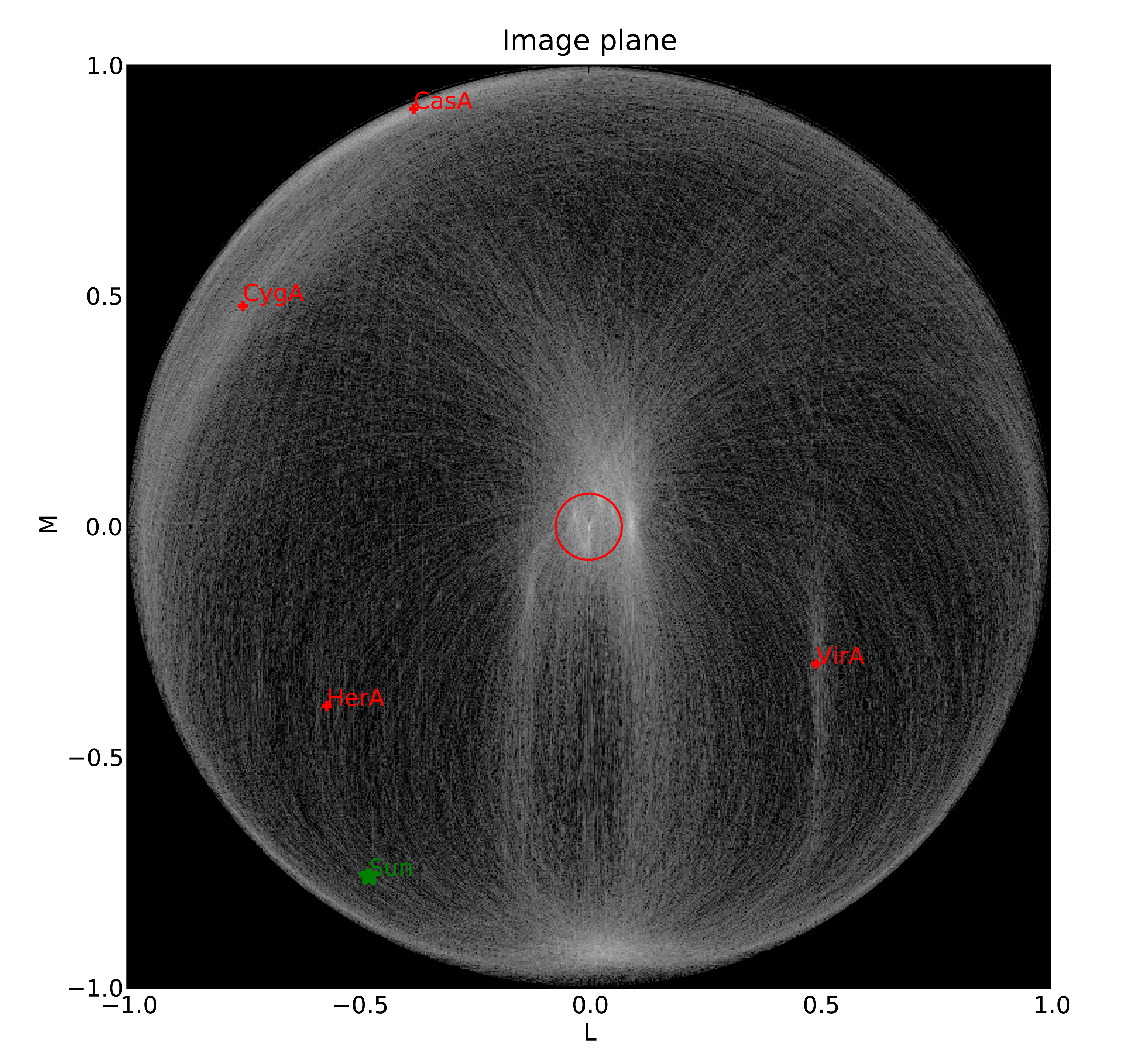
The Drawer is a useful algorithm that can be adopted to quickly inspect a MeasurementSet and investigate which sources are contributing to the visibilities. The software automatically converts the fringes seen in the visibilities to locations in the sky, having the advantage that (i) it works very well on the raw data and therefore it can be used before any calibration, (ii) it is very fast to recover spatial information on the half sphere centered on the phase center of the observation (one can generally generate an all sky plot in less than a few minutes). The concept behind the Drawer was already known and used in AIPS (task FRMAP).

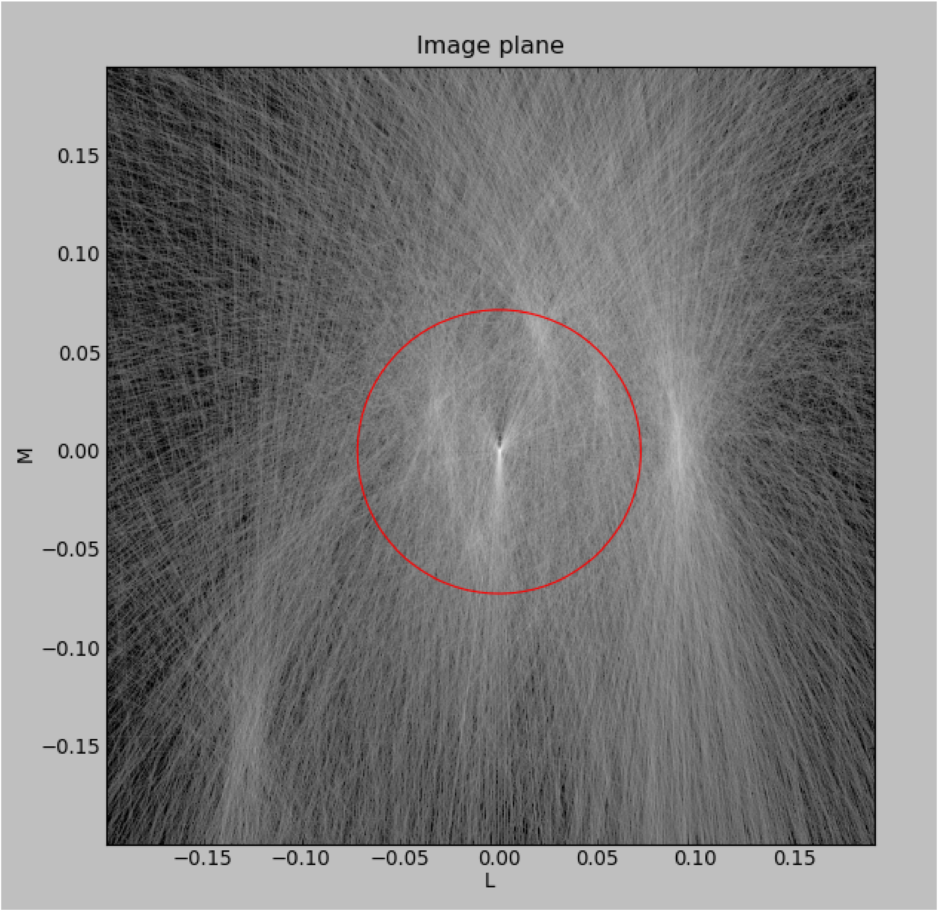
As the fringes “produced” by each individual baseline are rotating on the sky, each source modulates the visibility, depending on its distance from the phase center (far away sources give a higher fringe rate). The Drawer performs an FFT of the visibility of each given baseline in a particular timeslot, along the time axis, and finds the dominant frequency. From that value, and from the “speed” of the given baseline in the uv plane, it solves a simple equation and derives a line on the sky. Per baseline, it reflects all the possible places where the source producing the given detected modulation could be. The lines of all the baselines/timeslots are then gridded onto an image. The pixel values do not reflect the flux of the sources, but the log of the occurrence of fringe finding. The current version of the software does not deal with data chunks yet, i.e. it first reads the whole MS and puts the visibilities into memory. Therefore it performs quicker on averaged datasets containing a few channels.

Examples¶

Fig. 2 DrawMS is a simple algorithm that allows to quickly recover spatial information on the sources that have the brightest apparent flux. In this example, drawMS is run on the raw data of an observation of the Bootes field. One can clearly see the contribution from CasA, CygA, and TauA, while there is no direct contribution from the Sun.¶

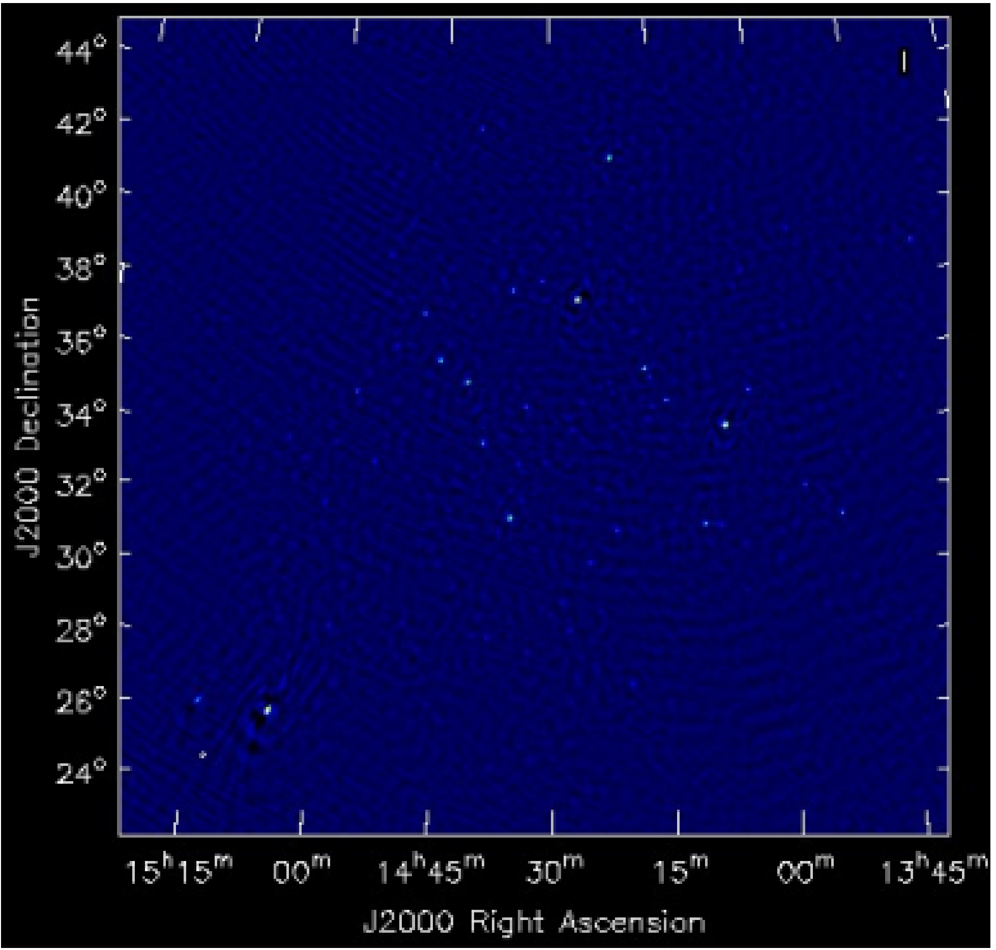
Fig. 3 A wide field of view image of the Bootes field which is computationally expensive to generate.¶

Fig. 4 In contrast to the image in Fig. 3, the output of drawMS takes a few minutes to generate. Line plots show the overdensities corresponding to real sources in the image.¶

Once you have initialized your work environment, you can access drawMS as

> drawMS -h

Options:
 --version             show program's version number and exit
 -h, --help            show this help message and exit

 * Necessary options:
   Won't work if not specified.

   --ms=MS             Input MS to draw [no default]

 * Data selection options:
   ColName is set to DATA column by default, and other parameters select
   all the data.

   --ColName=COLNAME   Name of the column to work on. Default is DATA. For
                       example: --ColName=CORRECTED_DATA
   --uvrange=UVRANGE   UV range (in meters, not in lambda!). Default is
                       0,10000000. For example: --uvrange=100,1000
   --wmax=WMAX         Maximum W distance. Default is 10000000.
   --timerange=TIMERANGE
                       Time selection range, in fraction of total observing
                       time. For example, --timerange=0.1,0.2 will select the
                       second 10% of the observation. Default is 0,1.
   --AntList=ANTLIST   List of antennas to compute the lines for. Default is
                       all. For example: --AntList=0,1,2 will plot 0-n, 1-n,
                       2-n
   --FillFactor=FILLFACTOR
                       The probability of a baseline/timeslot to be
                       processed. Default is 1.0. Useful when large dataset
                       are to be drawn. For example --FillFactor=0.1 will
                       result in a random selection of 10% of the data

 * Algorithm options:
   Default values should give reasonable results, but all of them have
   noticeable influence on the results

   --timestep=TIMESTEP
                       Time step between the different time chunks of which
                       the drawer does the fft. Default is 500.
   --timewindow=TIMEWINDOW
                       Time interval width centered on the time bin
                       controlled by --timestep. If not defined then it is
                       set to --timestep.
   --snrcut=SNRCUT     Cut above which the fringe is drawn. Default is 5.0.
   --maskfreq=MASKFREQ
                       When a fringe is found, it will set the fft to zero in
                       that 1D pixel range. Default is 2.0.
   --MaxNPeaks=MAXNPEAKS
                       Maximum number of fringes it will find per baseline
                       and timeslot. Default is 7.
   --NTheta=NTHETA     Number of angles in the l-m plane the algorithm will
                       solve for. Default is 20.

 * Fancy options:
   Plot NVSS sources, or make a movies.

   --RadNVSS=RADNVSS   Over-plot NVSS sources within this radius. Default is
                       0 (in beam diameter).
   --SlimNVSS=SLIMNVSS
                       If --RadNVSS>0, plot the sources above this flux
                       density. Default is 0.5 Jy.
   --MovieName=MOVIENAME
                       Name of the directory that contains the movie (.mpg),
                       the individual timeslots (.png), and the stack
                       (.stack.png). Each page correspond to the data
                       selected by --timewindow, separated by --timestep. For
                       example --MovieName=test will create a directory
                       "dMSprods.test". Default is None.

As explained in the help file, default values should give reasonable results, but all of them have noticeable influence on the results. However, some handy parameters that are often used are the following: ColName (DATA by default, or CORRECTED_DATA), FillFactor (less lines, but speedup the calculus), RadNVSS (to display the location of NVSS sources), MovieName (to generate a time-movie), and timewindow/timestep (see help file).

Here are a few examples of drawMS possible usage. For the plot shown in Fig. 3, on the raw data:

> /home/tasse/drawMS/drawMS --timerange=0.0,0.5 --ms=name.MS --FillFactor=0.5

The following command lets you make a movie of the line plots like the one shown in Fig. 3

drawMS --ms=name.MS --snrcut=3 --timestep=100 --timewindow=300 --uvrange=100,100000 --MovieName=test

Footnotes

1: This chapter is maintained by A. Shulevski and Valentina Vacca.
2: The script was written by George Heald and is available through the LOFAR GitHub repository.
3: For more information, consult this webpage.
4: This is due to the fact that the MS writer version used during those months was specifying the antenna mount as FIXED, and not as ALT-AZ, which is CASA friendly. To solve this problem, you can run the following taql command on your MS as taql ‘update <ms name>/ANTENNA set MOUNT=”X-Y” ‘
5: The SPLIT task will be deprecated in favour of the MSTRANSFORM task beginning with CASA v.4.1.0.
6: The script is available through the LOFAR GitHub repository.

Data inspection 1¶