Calibration with BBS 1 ¶

BBS is a software package that was designed for the calibration and simulation of LOFAR data. This section provides a practical guide to reducing LOFAR data with BBS. Do not expect a description of the optimal way to calibrate LOFAR data that works on all possible fields. Much still has to be learned about the reduction of LOFAR data. This chapter should rather be viewed as a written record of the experience gained so far, through the efforts of many commissioners and developers.

NOTE: the most common calibration scenarios can now be performed in DPPP, which is a lot faster (at least 10 times). Please first see if your calibration can be done with DPPP, see gain calibration with DPPP.

Overview¶

The sky as observed by LOFAR is the “true” sky distorted by characteristics of the instrument (station beam, global bandpass, clock drift, and so on) and the environment (ionosphere). The goal of calibration (and imaging) is to compute an accurate estimate of the “true” sky from the distorted measurements.

The influence of the instrument and the environment on the measured signal can be described by the measurement equation. Calibration involves solving the following inverse problem: Given the measured signal (observations) and a parameterized measurement equation (model), find the set of parameter values that minimizes the difference between the model and the observations.

The core functionality of BBS can conceptually be split into two parts. One part concerns the simulation of visibilities given a model. The other part concerns estimating best-fit parameter values given a model and a set of observed visibilities. This is an iterative procedure: A set of simulated visibilities is computed using the current values of the parameters. Then, the values of the parameters are adjusted to minimize the difference between simulated visibilities and observed visibilities, and an updated set of simulated visibilities is computed. This continues in a loop until a convergence criteria is met.

BBS has two modes of running. The first is to run as a stand-alone tool to calibrate one subband. If a single subband does not contain enough signal, BBS offers the possibility to use data from multiple subbands together for parameter estimation. This is called global parameter estimation. In this chapter, we will focus on the stand-alone version; only in section global parameter estimation we will treat the global solve.

As input, BBS requires an observation (one or more subbands / measurement sets), a source catalog, a table of initial model parameters (see section on instrument tables), and a configuration file (also called parset, see section example reductions) that specifies the operations that need to be performed on the observation as a whole. As output, BBS produces a processed observation, a table of estimated model parameters, and a bunch of log files.

Usage¶

To calibrate a single MS, execute the calibrate-stand-alone script on the command line:

> calibrate-stand-alone -f <MS> <parset> <source catalog>

The important arguments provided to the calibrate-stand-alone script in this example are:

<MS>, which is the name of the MS to process.
<parset>, which defines the reduction (see section example reductions).
<source catalog>, which defines a list of sources that can be used for calibration (see section source catalog).
The -f option, which overwrites stale information (the instrument table and sky model) from previous runs.

You can run the script without arguments for a description of all the options and the mandatory arguments, such as the -v option to get a more verbose output.

Source catalog¶

The source catalog / sky model defines the sources that can be used (referred to) in the reduction. It is a plain text file that is translated by the makesourcedb tool into a form that BBS can use. (Internally, the script converts the catalog file to a sourcedb by running makesourcedb on it, before starting BBS.)

A sky model can be created by hand using a text editor. Using tools like awk and sed, it is relatively straight-forward to convert existing text based catalogs into makesourcedb format. Various catalog files created by commissioners have been collected in a GitHub repository.

Alternatively, a catalog file in makesourcedb format can be created using the gsm.py tool. This tool extracts sources in a cone of a given radius around a given position on the sky from the Global Sky Model or GSM. The GSM contains all the sources from the VLSS, NVSS, and WENSS survey catalogs. See section GSM for more information about the GSM and gsm.py.

Below is an example catalog file for 3C196. In this example, 3C196 is modelled as a point source with a flux of 153 Jy and a spectral index of -0.56 with a curvature of -0.05212 at a reference frequency of 55.468 MHz.

# (Name,Type,Ra,Dec,I, ReferenceFrequency='55.468e6', SpectralIndex) = format
3C196, POINT, 08:13:36.062300, +48.13.02.24900, 153.0, , [-0.56, -0.05212]

Another example catalog file describes a model for Cygnus~A. It is modelled as two point sources that represent the Eastern and the Western lobe respectively, with a flux ratio of 1:1.25.

# (Name, Type, Ra, Dec, I) = format
CygA.E, POINT, 19:59:31.60000, +40.43.48.3000, 1.25
CygA.W, POINT, 19:59:25.00000, +40.44.15.7000, 1.0

For each source, values should be specified for the fields listed in the header line, in the same order. The only mandatory fields are: Name, Type, Ra, and Dec. The declination separators have to be dots, not colons, unless you want the declination to be interpreted as hours (i.e., multiplied by a factor 15).

If a field is left blank (e.g. the ReferenceFrequency in the 3C196 example above), the default value specified in the header line is used. If this is not available, then the application defined default value is used instead.

When a catalog contains sources defined by shapelets as well as point sources or Gaussian sources, it is easiest to create two catalog files (one containing the shapelet sources and one containing the rest). Using the append option of the makesourcedb tool, a single sourcedb containing all the sources can then be created and fed to the calibrate-stand-alone script using the sourcedb option.

For more information about the recognized fields, default values, and units, please refer to the makesourcedb documentation on the LOFAR wiki.

Gaussian sources¶

A Gaussian source can be specified as follows.

# (Name, Type, Ra, Dec, I, Q, U, V, ReferenceFrequency='60e6', SpectralIndex='[0.0]', MajorAxis, MinorAxis, Orientation) = format
sim_gauss, GAUSSIAN, 14:31:49.62,+13.31.59.10, 5,,,,,[-0.7], 96.3, 58.3, 62.6

Note that the header line beginning with “# (Name, …” must be a single line, and has been spread over multiple lines here for clarity (indicated by a backslash). There is a known issue about the definition of the Orientation: it’s defined relative to the north of some image and not relative to ‘true’ north. This is only relevant if the Gaussian is not symmetric, i.e. the major axis and minor axis differ, and you are transferring a Gaussian model component to another pointing over a large angular distance.

Spectral index¶

The spectral index used in the source catalog file is defined as follows:

\[{\rm \log}_{10}(S) = {\rm \log}_{10}(S_{0}) + c_{0} {\rm \log}_{10}\left(\frac{\nu}{\nu_{0}}\right) + c_{1}\left[{\rm \log}_{10}\left(\frac{\nu}{\nu_{0}}\right)\right]^{2} + \ldots + c_{n}\left[{\rm \log}_{10}\left(\frac{\nu}{\nu_{0}}\right)\right]^{n+1}\]

with \(\nu_{0}\) being the reference frequency specified in the ReferenceFrequency field, \(c_{0}\) the spectral index, \(c_{1}\) the curvature, and \(c_{2}, \ldots, c_{n}\) the higher order curvature terms. The SpectralIndex field should contain a list of coefficients \([c_{0}, \ldots, c_{n}]\).

Rotation measure¶

For polarized sources, Stokes \(Q\) and \(U\) fluxes can be specified explicitly, or implicitly by specifying the intrinsic rotation measure \(RM\), the polarization angle \(\chi_{0}\) at \(\lambda = 0\), and the polarized fraction \(p\).

In the latter case, Stokes \(Q\) and \(U\) fluxes at a wavelength \(\lambda\) are computed as:

\begin{align} Q(\lambda) &= p \; I(\lambda) \; \cos(2 \chi (\lambda)) \\ U(\lambda) &= p \; I(\lambda) \; \sin(2\chi(\lambda)) \\ \chi(\lambda) &= \chi_{0} + RM \; \lambda^{2} \end{align}

Here, \(I(\lambda)\) is the total intensity at wavelength \(\lambda\), which depends on the spectral index of the source.

The intrinsic rotation measure of a source can be specified by means of the field RotationMeasure. The polarization angle \(\chi_{0}\) at \(\lambda = 0\) and the polarized fraction \(p\) can be specified in two ways:

Explicitly by means of the fields PolarizationAngle and PolarizedFraction.
Implicitly, by means of the fields Q, U, and ReferenceWavelength.

When specifying \(Q\) and \(U\) at a reference wavelength \(\lambda_{0}\), the polarization angle \(\chi_{0}\) at \(\lambda = 0\), and the polarized fraction \(p\) will be computed as:

\begin{align} \chi_{0} &= \frac{1}{2}\tan^{-1}(\frac{U}{Q}) - \lambda_{0}^2 \; RM \\ p &= \frac{\sqrt{(Q^{2} + U^{2})}}{I(\lambda_{0})} \end{align}

Here, \(I(\lambda_{0})\) is the total intensity at reference wavelength \(\lambda_{0}\), which depends on the spectral index of the source. Note that the reference wavelength \(\lambda_{0}\) must be \(>0\) if the source has a spectral index.

GSM¶

The Global Sky Model or GSM is a database that contains the reported source properties from the VLSS, WENSS and NVSS surveys. The gsm.py script can be used to create a catalog file in makesourcedb format (see Source catalog) from the information available in the GSM. As such, the gsm.py script serves as the interface between the GSM and BBS.

A catalog file created by gsm.py contains the VLSS sources that are in the field of view. For every VLSS source, counterparts in the other catalogs are searched and associated depending on criteria described below. Spectral index and higher-order terms are fitted according to equation in section Spectral index.

On CEP, there is a GSM database instance and is loaded with all the sources and their reported properties from the VLSS, WENSS and NVSS surveys. The WENSS survey is actually split up into two catalogs according to their frequencies: A main (\(\delta \leq 75.8\), \(\nu=325\) MHz) and a polar (\(\delta \geq 74.5\), \(\nu=352\) MHz) part. The VLSS and NVSS surveys are taken at 73.8 MHz and 1400 MHz, respectively.

The python wrapper script gsm.py can be used to generate a catalog file in makesourcedb format and can be run as:

> gsm.py outfile RA DEC radius [vlssFluxCutoff [assocTheta]]

The input arguments are explained in Table 4. The arguments RA and DEC can be copy-pasted from the output of ‘msoverview’ to select the pointing of your observation. A sensible value for radius is 5 degrees.

Table 4 The parameters and criteria that are used for creating the initial Global Sky Model.¶
Parameter	Unit	Description
outfile	string	Path to the makesourcedb catalog file. If it exists, it will be overwritten.
RA, DEC	degrees	Central position of conical search.
radius	degrees	Extent of conical search.
vlssFluxCutoff	Jy	Minimum flux of VLSS source in outfile. Defaults to 4 Jy.
assocTheta	degrees	Search radius centered on VLSS source for which counterparts are searched. Defaults to 10 arcsec taking into account the VLSS resolution of 80 arcsec.

The gsm.py script calls the function expected_fluxes_in_fov() in gsmutils.py that does the actual work. It makes a connection to the GSM database and selects all the VLSS sources that fulfill the criteria. The area around every found VLSS source (out to radius assocTheta) is searched for candidate counterparts in the other surveys. The dimensionless distance association parameter, \(\rho_{i,\star}\), is used to quantify the association of VLSS source-candidate counterpart further. It weights the positional differences by the postion errors of the pair and follows a Rayleigh distribution (De Ruiter et al., 1977). A value of \(3.717\) corresponds to an acceptance of missing 0.1% genuine source associations (Scheers, 2011). The dimensionless radius is not an input argument to gsm.py, but it is to the above mentioned function. For completeness, we give its definition below:

\[\rho_{i,\star} \equiv \sqrt{ \frac{(\alpha_i \cos \delta_i - \alpha^{\star} \cos \delta^{\star})^2}{\sigma^2_{\alpha_i} + \sigma^2_{\alpha^{\star}}} + \frac{(\delta_i -\delta^{\star})^2}{\sigma^2_{\delta_i} + \sigma^2_{\delta^{\star}}}}.\]

Here the sub- and superscripts \(\star\) refers to the VLSS source and \(i\) to its candidate counterpart in one of the other surveys.

After being associated (or not), the corresponding fluxes and frequencies are used to fit the spectral-index and higher-order terms according to the equation in section Source catalog. Therefore, we use the python numpy.poly1d() functions. If no counterparts were found a default spectral index of \(-0.7\) is assumed.

Another optional argument when calling the function expected_fluxes_in_fov() in gsmutils.py is the boolean storespectraplots. When true and not performance driven, this will plot all the spectra of the sources in the catalog file, named by their VLSS name.

Special cases¶

There might be cases that a VLSS source has more than one WENSS counterpart. This might occur when the mutiple subcomponents of a multicomponent WENSS source are associated to the VLSS source. WENSS sources that are flagged as a subcomponent (‘C’) are omitted in the inclusion. Only single component WENSS sources (‘S’) and multicomponent WENSS sources (‘M’) are included in the counterpart search.

Generating a higher resolution skymodel¶

The skymodel generated using gsm.py is limited in angular resolution due to the \(80^{\prime \prime}\) resolution of the VLSS. Users in need of a higher resolution skymodel can generate a model of the sky using data from The GMRT Sky Survey - Alternative Data Release (TGSS-ADR). Skymodels generated using TGSS-ADR have an angular resolution of \(20^{\prime \prime}\). Information about the survey and the data products provided by TGSS-ADR are described in detail in Intema et al (2017).

You can generate a skymodel from TGSS-ADR as

# 3C295 = (212.83,52.21)
ra=212.83
dec=52.21
radius=5
out=skymodel.txt
wget -O $out 'http://tgssadr.strw.leidenuniv.nl/cgi-bin/gsmv2.cgi?coord=${ra},${dec}\&radius=${radius}\&unit=deg\&deconv=y

The above set of commands will generate the file skymodel.txt which contains all TGSS-ADR sources within a 5 degree radius from the specified coordinate (212.83,52.21). Note that the coordinates are in degrees and in the J2000 epoch.

Instrument tables¶

When calibrating, we try to estimate parameters in the measurement equation. The values of these model parameters are stored in a so-called “parmdb” (table). Usually, this parmdb is stored inside a measurement set and is called instrument. To inspect or create a parmdb, use the command parmdb. To view the contents of a parmdb, use the tool parmdbplot.py (see section Inspecting the solutions).

A parmdb can contain two sorts of parameters: normal parameters that are both time and frequency dependent, and default parameters that are neither frequency nor time dependent. The default parameters can be used as fallback if a model parameter is not known, but they can also be used in some schemes for transferring solutions, see section on gain transfer below.

Before even starting the actual BBS, there need to be values in the parmdb, because they are used as starting values by BBS 2. For gains (Gain and DirectionalGain), the default starting value of \(0\) is not adequate. For this reason, the calibrate-stand-alone script implicitly creates a default parmdb that contains initial values of \(1\) for these parameters.

Please note that if you create your own parmdb, you will almost always want to include the default adddef commands listed below to set the correct defaults for Gain, DirectionalGain. Otherwise, estimating these parameters will not work correctly. The default parameters are automatically created if you use calibrate-stand-alone with the option -f or –replace-parmdb. To set default values in a parmdb manually, use the following commands in parmdbm.

adddef Gain:0:0:Ampl  values=1.0
adddef Gain:1:1:Ampl  values=1.0
adddef Gain:0:0:Real  values=1.0
adddef Gain:1:1:Real  values=1.0
adddef DirectionalGain:0:0:Ampl  values=1.0
adddef DirectionalGain:1:1:Ampl  values=1.0
adddef DirectionalGain:0:0:Real  values=1.0
adddef DirectionalGain:1:1:Real  values=1.0

Model¶

As already mentioned, BBS consists of two parts: a part to solve equations and a part to simulation of visibilities given a sky model. This section is about the latter. BBS uses the measurement equation, which is an equation that describes all effects that happen to the signal that was sent by the sky, before they are captured in your data. All these effects are Jones matrices: \(2 \times 2\) matrices that work on the two components (the two polarizations) of your data. An important thing to note is that these Jones matrices do not commute: the order in which they are matters.

The most commonly used effects that BBS can handle are given in Table 5, in the order that they are applied (from sky to antenna). The direction dependent effects are different for each patch you specify in your source model.

Table 5 Effects that BBS handles. The first half are direction dependent effects (DDEs), which means that the effect is different for each patch. The bottom effects are direction independent effects (DIEs).¶
Effect	Description	Jones matrix
ScalarPhase	A phase that is equal for both dipoles	\(\left( \begin{smallmatrix} e^{\alpha_p}& 0\\ 0 & e^{\alpha_p} \end{smallmatrix}\right)\)
Rotation 18	Faraday Rotation without frequency dependency	\(\left( \begin{smallmatrix} \cos(\alpha_p) & -\sin(\alpha_p)\\ \sin(\alpha_p) & \cos(\alpha_p) \end{smallmatrix}\right)\)
FaradayRotation 19	Faraday Rotation, \(\rho_p=\alpha_p\cdot\text{(channel wavelength)}^2\)	\(\left( \begin{smallmatrix} \cos(\rho_p) & -\sin(\rho_p)\\ \sin(\rho_p) & \cos(\rho_p) \end{smallmatrix}\right)\)
Directional TEC	TEC (ionosphere), \(\phi_p=\frac{-8.44797245\cdot 10^9\alpha_p}{\textrm{channel frequency}}\)	\(\left( \begin{smallmatrix} e^{\phi_p} & 0\\ 0 & e^{\phi_p} \end{smallmatrix}\right)\)
Beam 20	The LOFAR beam model	See section on Beam model
DirectionalGain	Directional gain	\(\left( \begin{smallmatrix} \alpha:0:0:p & \alpha:0:1:p\\ \alpha:1:0:p & \alpha:1:1:p \end{smallmatrix}\right)\)
CommonScalarPhase	Scalar phase	\(\left( \begin{smallmatrix} e^\alpha & 0\\ 0 & e^\alpha \end{smallmatrix}\right)\)
CommonRotation	Rotation	\(\left( \begin{smallmatrix} \cos(\alpha) & -\sin(\alpha)\\ \sin(\alpha) & \cos(\alpha) \end{smallmatrix}\right)\)
TEC	TEC (ionosphere), \(\phi=\frac{-8.44797245\cdot 10^9\alpha}{\text{channel frequency}}\)	\(\left( \begin{smallmatrix} e^\phi & 0\\ 0 & e^\phi \end{smallmatrix}\right)\)
Gain	Gain	\(\left( \begin{smallmatrix} \alpha:0:0 & \alpha:0:1\\ \alpha:1:0 & \alpha:1:1 \end{smallmatrix}\right)\)
Clock	Clock, \(\phi=\alpha\cdot 2\pi\cdot\text{channel frequency}\)	\(\left( \begin{smallmatrix} e^\phi & 0\\ 0 & e^\phi \end{smallmatrix}\right)\)

The two most commonly used effects, Gain and DirectionalGain, have only one option: Phasors. When set to True (or T), the gains are expressed like \(A\cdot e^{i\phi}\), otherwise they are specified in the form \(a + b\cdot i\). While mathematically equivalent, this does make a difference because the solver in BBS solves for real variables. When you are solving for phases or amplitudes only, it is necessary to specify Phasors = True. Specify this like

Model.Gain.Phasors = T

For configuration of the beam model that is used, see section Beam model.

Beam model¶

The beam model tries to emulate all kinds of distortions to the signal that are caused by the beam of the station. These effects are split into two parts: the element beam, which is the response of a single dipole, and the array factor, which emulates the effect of combining the signal of the many dipoles in a station. In HBA, the array factor model also models the effect of the analogue tile beam former.

To have a look at different elements of the beam, you can specifically use only the element beam or only the array factor (if you don’t know the details, you need both the element beam and the array factor, which is the default). The options are

Model.Beam.Mode = ELEMENT       # only element beam
Model.Beam.Mode = ARRAY_FACTOR  # only array factor
Model.Beam.Mode = DEFAULT       # both element beam and array factor (default)

The tile beam former in the HBA tiles forms a beam for a certain reference frequency. When modeling this beam, the beam model should of course do this for the same frequency. Usually, this works automatically: the reference frequency is stored in the measurement set. Things are different when you compress a number of subbands as channels into one measurement set (usually done with DPPP). Then each ‘channel’ was beamformed at a different reference frequency. In this case, the reference frequency is only right for one of the ‘channels’. To handle this case well, there is an option that tells the beam model to use the channel frequency (which is usually the center frequency of the compressed subband). This option is

Step.Solve.Model.Beam.UseChannelFreq = T

Note that the beam model is a direction dependent effect like any other in BBS. That means that over a patch, the beam is assumed to be constant (it is evaluated at the centroid of the patch). This may change in the future.

Solver¶

BBS performs parameter estimation on the measurement equation to find parameters that best match the observed visibilities. To improve signal to noise, one can assume that the parameters are constant for a number of time samples or a number of frequencies. In this way, there are more measurements available to estimate the same parameter. To specify these, use Step.<name>.Solve.CellSize.Time and Step.<name>.Solve.CellSize.Freq. The unit of CellSize.Time is number of time slots, so CellSize.Time=1 corresponds to the correlator integration time. If CellSize.Time=0, one solution is calculated for the entire scan.

The underlying solver is a Levenberg-Marquardt solver. Several parameters exist to this solver, however the defaults should be fine.

Example reductions¶

The sequence of operations that BBS will perform on the data are defined in a configuration or parset file 3. The BBS documentation on the LOFAR wiki documents all the options (see the LOFAR wiki), and it is highly recommended that you obtain a hard-copy of this for future reference.

A BBS parset file consists of two sections: The Strategy section, which defines the operations (or steps) to be carried out, and the Step section, which defines the details of each step. The following sections describe a few typical reductions along with the corresponding parset.

The parsets shown in the following sections are intentionally verbose. Often, default settings have been included for clarity. For example, the default input column is DATA. The line Strategy.InputColumn = DATA is therefore redundant and can be left out.

Simulation¶

Given a source catalog and (optionally) a table of model parameters, BBS can be used to compute simulated uv-data (without noise) 4. Simulated data can sometimes be useful as a debugging aid. Imaging simulated data can provide an impression of what you would expect to see with an ideal telescope under ideal conditions and without noise. Comparing observed data to simulated data can provide useful clues, although in practice this is limited to cases where the signal to noise ratio of the observed data is high.

Simulated data produced by BBS (or any other software package) can also be used as model data during calibration using the same parset syntax as described in section Pre-computed visibilities.

An example parset file 5 to simulate {it uv}-data for all the sources in the source catalog is shown below.

# simulation.parset
Strategy.InputColumn = DATA
Strategy.TimeRange = []
Strategy.Baselines = *&
Strategy.ChunkSize = 100
Strategy.Steps = [predict]
Step.predict.Operation = PREDICT
Step.predict.Model.Sources = []
Step.predict.Output.Column = MODEL_DATA

Gain calibration (direction-independent)¶

The following parset 6 describes a direction independent gain calibration. The meaning of each parameter is the same as in section Simulation unless otherwise stated. Enabling / disabling of model components can be either done by a short-hand T and F which is equivalent to explicit True and False.

# uv-plane-cal.parset
Strategy.InputColumn = DATA
Strategy.TimeRange = []
Strategy.Baselines = *&
Strategy.ChunkSize = 100
Strategy.Steps = [solve, correct]

Step.solve.Operation = SOLVE
Step.solve.Model.Sources = [3C196]
Step.solve.Model.Gain.Enable = T
Step.solve.Solve.Parms = ["Gain:0:0:*", "Gain:1:1:*"]
Step.solve.Solve.CellSize.Freq = 0
Step.solve.Solve.CellSize.Time = 1
#Step.solve.Model.Beam.Enable = True  <-uncomment if you want to apply the beam

Step.correct.Operation = CORRECT
Step.correct.Model.Gain.Enable = T
Step.correct.Output.Column = CORRECTED_DATA
#Step.correct.Model.Beam.Enable = True <-uncomment if you want to apply the beam

The CORRECT step performs a correction of the uv-data for a particular direction. This can be done for exactly one source from the skymodel. If Model.Sources contains multiple sources, BBS will throw an exception, because it cannot correct for more than one direction at a time.

BBS also accepts an empty source list in the CORRECT step. In that case it will correct for the phase center direction of the MS. This does then, of course, not include direction dependent effects such as DirectionalGain, DirectionalTEC, et cetera, which are inherently bound to a patch name and therefore can only be corrected for if a patch name is specified. This implicit behaviour must be kept in mind when correcting your data.

Note that a CORRECT step cannot be “undone”. If a CORRECTED_DATA column is used for further calibration later on, one has to be aware of the consequences. For example, if in the first correct the beam was enabled, this prevents proper use of the beam in the following steps 7.

Gain calibration (direction-dependent) with source subtraction¶

This section has been adapted from a document written by Annalisa Bonafede. In the following, we report the parset 8 file and skymodel used for the subtraction of Cas A and Cyg A from the observation of the radio source 3C380.

The parset includes the following steps:

Solve for the gain in the direction of each source in the source catalog.
Subtract the sources CygA.E, CygA.W, and CasA, each with their own individual gain.

Correct the data for the gain in the direction of 3C380 (the target).

# image-plane-cal.parset
#

Strategy.ChunkSize = 100
Strategy.Steps = [solve, subtract, correct]

Step.solve.Operation = SOLVE
Step.solve.Model.DirectionalGain.Enable = T
Step.solve.Solve.Parms = ["DirectionalGain:0:0:*","DirectionalGain:1:1:*"]
Step.solve.Solve.CellSize.Freq = 0
Step.solve.Solve.CellSize.Time = 5

Step.subtract.Operation = SUBTRACT
Step.subtract.Model.Sources = [CygA.E, CygA.W, CasA]
Step.subtract.Model.DirectionalGain.Enable = T

Step.correct.Operation = CORRECT
Step.correct.Model.Sources = [3C380]
Step.correct.Model.DirectionalGain.Enable = T
Step.correct.Output.Column = CORRECTED_DATA

The source catalog used for calibration is reported below 9

############################################################
# 3C380-bbs.skymodel
# (Name, Type, Ra, Dec, I, ReferenceFrequency, SpectralIndex) = format

CygA.E, POINT, 19:59:29.99, +40.43.57.53, 4421, 73.8e6, [-0.7]
CygA.W, POINT, 19:59:23.23, +40.44.23.03, 2998, 73.8e6, [-0.7]
CasA, POINT, 23:23:24.0, +58.48.54.0, 20000
3C380, POINT, 18:29:31.8, +48.44.46.0, 1, 178.e6, [-0.7]

The flux of 3C380 has been set to the arbitrary value of 1 Jy. Its spectral index has been roughly estimated by comparing VLSS and 3C flux. The subtraction can also be performed without specifying the correct flux of the sources and determining the flux of the target source with self calibration.

The resulting image in shown in Fig. 19, compared to the map obtained without subtraction.

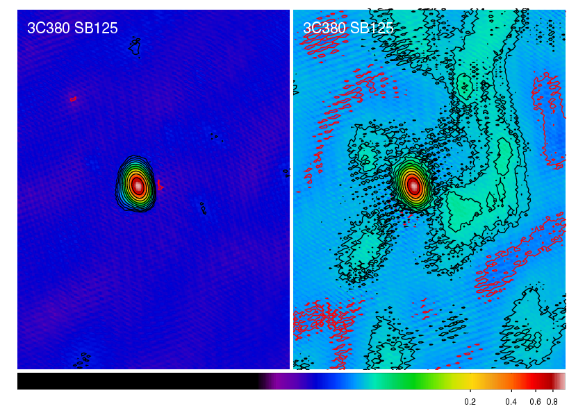
Fig. 19 The radio source 3C380 imaged by LOFAR at 135~MHz (observation ID L2010_08567). Left panel: Self calibration has been applied with directional-gain correction and subtraction of CygA and CasA. Right panel: Self calibration has been applied without correction. The lowest contour level is at 3 mJy \(\mathrm{beam}^{-1}\); subsequent contour levels are spaced by factors of \(\sqrt{2}\). The resolution is \(83.29" \times 59.42"\). The negative contour is in red.¶

Tweaking BBS to run faster¶

BBS can take a long time to calibrate your huge dataset. Luckily, there are some ways to tune it. You have to know a bit about how BBS works to do this.

BBS views the data as a grid of time slots times vs channels (see Fig. 20). A solution cell is defined as the number of timeslots times the number of channels on which a constant parameter solution is computed. For example, if you specify CellSize.Freq = 1, a different solution is computed for every channel independently. In Fig. 20, the solution cells are outlined with blue lines.

Because the evaluation of the model is computationally expensive, and a lot of intermediate results can be reused, the model is evaluated for a number of cells simultaneously. There is a trade-off here: if one cell would converge to a solution very slowly, the model is evaluated for all the cells in the cell chunk, even the ones that have converged. The number of cells in a cell chunk is specified by CellChunkSize, which specifies the number of solution cells in the time direction. Dependent on the amount of frequency cells, a value of CellChunkSize = 10 – 25 could be good.

First, BBS loads a lot of timeslots into memory. The amount of timeslots is specified by ChunkSize. If you specify ChunkSize = 0 then the whole MS will be read into memory, which will obviously not work if your data is 80 Gb large. Depending on the number of baselines and channels, usually 100 is a good choice. Monitor the amount of memory that is used (for example by running top) to see if you’re good. The ChunkSize should be an integer multiple of CellSize.Time \(\times\) CellChunkSize, so that in every chunk the same number of cell chunks are handled and all cell chunks have the same size.

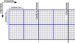
Fig. 20 The different solve domains and chunk parameters for BBS. In this example, CellSize.Time=8, CellSize.Freq=8, ChunkSize=32, CellChunkSize=2 (do not use these values yourself, they are probably not good for actual use).¶

Multithreading¶

BBS can do a bit of multithreading. Be warned in advance that if you use \(N\) threads, BBS will most likely not run \(N\) times faster. Again, a bit of tweaking may be necessary.

The multithreading is done on solve part, not on the model building part. So it works only on problems that are ‘solve-dominated’. The multithreading is performed over the solution cells. For this to give any speedup, there need to be at least as many solution cells as the number of threads. You usually get a decent speed-up if the number of solution cells is about 5–6 times the number of threads. So if you solve over all frequencies (the number of frequency cells is 1), CellChunkSize = 5 \(\times\) nThreads should give you some speedup.

You can instruct calibrate-stand-alone 10 to run with multithreading with the parameter -t or –numthreads

calibrate-stand-alone --numthreads 8 <MS> <parset> <source catalog>

Global parameter estimation¶

BBS was designed to run on a compute cluster, calibrating across multiple subbands which reside on separate compute nodes. BBS consists of three separate executables: bbs-controller, bbs-reducer, and bbs-shared-estimator. The bbs-controller process monitors and controls a set of bbs-reducer processes, and possibly one or more bbs-shared-estimator processes. Each subband is processed by a separate bbs-reducer process. When working with calibrate-stand-alone, the script actually launches one bbs-reducer for you. To setup a calibration across subbands, the script calibrate can be used, which sets up the appropriate processes on different nodes.

Each bbs-reducer process computes a set of equations and sends this to the bbs-shared-estimator process assigned to the group it is part of. The bbs-shared-estimator process merges the set of equations with the sets of equations it receives from the other bbs-reducer processes in the group. Once it has received a set of equations from all the bbs-reducer in its group, the bbs-shared-estimator process computes a new estimate of the model parameters. This is sent back to all bbs-reducer processes in the group and the whole process repeats itself until convergence is reached.

Setting up your environment¶

Before using the distributed version of BBS, you will have to set up a personal database. In principle, this needs to be done only once. You only have to recreate your database when the BBS SQL code has changed, for example to support new functionality. Such changes are kept to a minimum.

Also, on each lce or locus node that you are going to use you need to create a working directory. Make sure you use the same path name on all the nodes . This has to be done only once.

The distributed version of BBS requires a file that describes the compute cluster (an example of such a file is cep1.clusterdesc 11) and a configuration or parset 12 file that describes the reduction.

For each MS that we want to calibrate it is necessary to create a vds file that describes its contents and location. This can be done by running the following command

> makevds cep1.clusterdesc <directory>/<MS>

After this, all vds files need to be combined into a single gds file, ready for calibration and/or imaging. This is done by typing

> combinevds <output file>.gds <vds file 1> [<vds file 2> ...]

Instead of specifying the list of input vds files, you could type *.vds. Note that the combine step is required even if we want to calibrate a single subband only, although normally you would calibrate a single subband using the stand-alone version of BBS.

Usage¶

To calibrate an observation with the distributed version of BBS on the Groningen cluster, execute the calibrate script on the command line

> calibrate -f --key <key> --cluster-desc ~/imaging.clusterdesc --db ldb001 --db-user postgres <gds file> <parset> <source catalog> <working directory>

which is a single command, spread over multiple lines, as indicated by a backslash. The important arguments provided to the calibrate script in this example are:

<key>, which is a single word that identifies the BBS run. If you want to start a BBS run while another run is still active, make sure that the runs have different keys (using this option).
<gds file>, which contains the locations of all the MS (subbands) that constitute the observation. It should be given here by its full path, for example /data/scratch/\(<\)>`/\(<\)>`.
<parset>, which defines the reduction (see section Example reductions).
<source catalog>, which defines a list of sources that can be used for calibration (see section Source catalog).
<working directory>, which is the working directory where BBS processes will be run and where the logs will be written (usually /data/scratch/<user name>). It should be created on each compute node that you intend to use. You can use the cexec command for this (see section Logging on to CEP3).
The -f option, which overwrites stale information from previous runs.

You can run the calibrate script without arguments for a description of all the options and the mandatory arguments. You can also use the -v option to get a more verbose output. Note that the arguments of calibrate are very much like 13 those of calibrate-stand-alone.

The calibrate script does not show progress information, which makes it difficult to estimate how long a BBS run will take to complete. One way around this is to log on to one of the compute nodes where BBS is processing, change to your local working directory, and monitor one of the bbs-reducer log files. These log files are named <key>_-kernel_-<pid>.log. The default key is default, and therefore you will often see log files named e.g. default_-kernel_-12345.log. The following command will print the number of times a chunk of visibility data was read from disk:

> grep “nextchunk” default_kernel_12345.log | wc -l

You can compute the total number of chunks by dividing the total number of time stamps in the observation by the chunk size specified in the parset (Strategy.ChunkSize). Of course, if you make the chunk size large, it may take BBS a long time to process a single chunk and this way of gauging progress is not so useful. Generally, it is not advisable to use a chunk size larger than several hundreds of time samples. This will waste memory. A chunk size smaller than several tens of time stamps is also not advisable, because it leads to inefficient disk access patterns.

Defining a global solve¶

Solving across multiple subbands can be useful if there is not enough signal in a single subband to achieve reasonable calibration solutions, i.e. the phase and amplitude solutions look more or less random. Basically, there should be enough source flux in the field for calibration. Of course, one first has to verify that the sky model used for calibration is accurate enough, because using an inaccurate sky model can also result in bad calibration solutions.

To enable global parameter estimation, include the following keys in your parset. Note that the value of the Step.<name>.Solve.CalibrationGroups key is just an example. This key is described in more detail below

Strategy.UseSolver = T
Step.<name>.Solve.CalibrationGroups = [3,5]

The Step.<name>.Solve.CalibrationGroups key specifies the partition of the set of all available subbands into separate calibration groups. Each value in the list specifies the number of subbands that belong to the same calibration group. Subbands are ordered from the lowest to the highest starting frequency. The sum of the values in the list must equal the total number of subbands in the gds file. By default, the CalibrationGroups key is set to the empty list. This indicates that there are no interdependencies and therefore each subband can use its own solver. Global parameter estimation will not be used in this case (even if Strategy.UseSolver = T).

When using global parameter estimation, it is important to realize that drifting station clocks and the ionosphere cause frequency dependent phase changes. Additionally, due to the global bandpass, the effective sensitivity of the telescope is a function of frequency. Therefore, at this moment, it is not very useful to perform global parameter estimation using more than about 1–2 MHz of bandwidth (5–10 consecutive subbands).

A few examples of using global parameter estimation with 10 bands would be:

Estimate parameters using all bands together:

Step.<name>.Solve.CalibrationGroups = [10]

Estimate parameters for the first 5 bands together, and separately for the last 5 bands together
```
Step.<name>.Solve.CalibrationGroups = [5,5]
```
Do not use global parameter estimation (even if Strategy.UseSolver = T)
```
Step.<name>.Solve.CalibrationGroups = []
```
Estimate parameters for band 0 separately, bands 1–3 together, bands 4–5 together, and bands 6–9 together (note that 1+3+2+4=10, the total number of subbands in our example)
```
Step.<name>.Solve.CalibrationGroups = [1,3,2,4]
```

Pre-computed visibilities¶

Diffuse, extended sources can only be approximately represented by a collection of point sources. Exporting clean-component (CC) models from catalogues (e.g. VLSS, WENSS) or first iteration major cycle selfcal images tend to contain many CCs, ranging up to 50,000. By using casapy2bbs.py these can be imported into a BBS catalog file, but processing these can take long and memory requirements might not even allow their usage at all. 14

An alternative lies in (fast) Fourier transforming model images directly into uv-data columns. These can then be used in BBS as model data. The import can be done with a tool called addUV2MS.

The first argument is the MS to which the uv-data is to be added. The second argument is a CASA image (extension .model). The filename of the image is stripped of its leading path and file extension. This is then the column name it is identified by in the parset, and can be seen in the MS. For example:

> addUV2MS -w 512 L24380SB030uv.MS.dppp.dppp $HOME/Images/3C196_5SBs.model

This will create a column of name 3C196_5SBs, containing the uv-data FFT’ed from this model image, using 512 w-projection planes. You can run addUV2MS multiple times with different images, or also with several images as additional command arguments, to create more than one uv-data column. While this works in principle with normal images, it is advisable to use clean component model images generated by CASA.

A few notes of caution though:

The image must have the same phase center as the MS, because the internal CASA-routine which is used, does not do any phase shifting.
For wide field images you should set an appropriate value for the number of w-planes used in the w-projection term (default=128).
Direction dependent effects cannot be handled for “large” images. This means the image has to be small on the scale over which the direction dependent effects change.
addUV2MS temporarily overwrites the frequency in the input images to match that in the MS. It restores the original frequency, but only one (multi-frequency channel images aren’t supported). Aborting the run may leave you then with a model image having an incorrect frequency entry.
Successive runs with the same input model image will overwrite the data in the respective column.

The column name generated by addUV2MS can be used in the BBS parset as:

Step.<name>.Model.Sources = [@columnname]

You can use casabrowser to find out which data columns are available in a given MS. Be careful about dots in the filename, and verify that your model refers to the name of the created column. Running addUV2MS -h will give you more information about its usage.

You can use cexecms to add model uv-data to more than one MS, for example:

> cexecms "addUV2MS -w 512 <FN> $HOME/Images/3C1965_SBs.model" "/data/scratch/pipeline/L2011_08175/*"

Inspecting the solutions¶

You can inspect the solutions using the python script parmdbplot.py. To start parmdbplot.py from the command line, you should first initialize the lofar environment (see Setting up your working environment). Then you can type, for example:

> parmdbplot.py SB23.MS.dppp/instrument/

The first thing you should see after starting the script should be the main window (see Fig. 21). Here you can select a set of parameters of the same type to be plotted together in a single plot. Note that some features will not be available if you select multiple parameters. Parmdbplot is able to properly handle the following solution types: Gain, DirectionalGain, CommonRotationAngle, RotationAngle, CommonScalarPhase, ScalarPhase, Clock, TEC, RM. The last three (Clock, TEC and RM) are properly converted into a phase – they are stored differently in the parmdb internally.

The “Use resolution” option is best left unchecked. If it is checked, the plotter tries to find a resolution that will yield a \(100 \times 100\) grid in \(\mathrm{frequency} \times \mathrm{time}\). Usually, you just want to use the sampling intervals that are present in the parmdb. In that case, leave the box unchecked.

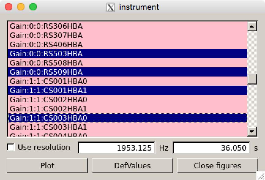
Fig. 21 The main window of parmdbplot.¶

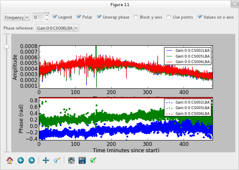
Fig. 22 The plot window of parmdbplot.¶

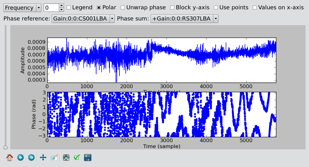
Fig. 23 The plot window of parmdbplot with a phase sum.¶

Once you click the “Plot” button, a window similar to the Fig. 22 should pop up. We discuss the controls on the top of the window from left to right. The first is a drop down box that allows you to select the axis (frequency, time) to slice over. By default, this is set to frequency, which means that the x-axis in the plot is time and that you can step along the frequency axis using the spin control (the second control from the left).

The “Legend” checkbox allows you turn the legend on or off (which can be quite large and thus obscure the plot, so it is off by default). The “Polar” checkbox lets you select if the parameter value is plotted as amplitude/phase (the default) or real/imaginary. The “Unwrap phase” checkbox will turn phase unwrapping on or off. The button “Block y-axis” is useful when stepping over multiple frequency solutions: if checked, the y-scale will remain the same for all plots. “Use points” can be checked if you want points (instead of lines) for amplitude plots.

The last checkbox lets you choose the unit for the x-axis. By default, it is the sample number. If you chose, in the main window, to use a time resolution of 2 seconds, then the number 10 on the x-axis means \(10 \times 2 = 20\) seconds. If you enable “Values on x-axis”, it will show the number of minutes since the start of the observation.

The Phase reference drop down box allows you to select the parameter used as the phase reference for the phase plots (the phase reference is only applied in amplitude/phase mode).

When the phase reference is set, one can use the phase sum drop-down menu (see Fig. 23). This menu allows the user to select among all the other parameters related to the same antenna and add the phases to those plotted. All the selected phases are referenced to the “phase reference” antenna. This procedure is useful if one solves for Phase and Clock (or TEC) and wants to look at the global phase effect. Note that the phase effects are just added together with not specific order. This is only physically correct if the effects commute.

The slider on the left of the plots allows you to make an exponential zoom to the median value of amplitude plots. This can be helpful if you have one outlier in the solution which sets the scale to 1000 when you are actually interested in the details around 0.001.

The controls on the bottom of the window are the default matplotlib controls that allow you to pan, zoom, save the plot, and so on.

For a quick overview of solutions, and to compare lots of solutions at a glance, you can also use the solplot.py 15 script by George Heald:

>solplot.py -q *.MS/instrument/

Running the script with -h will produce an overview of possible options.

The global bandpass¶

This section describes estimates of the global bandpass for the LBA band and HBA bands. The bandpass curves were estimated from the BBS amplitude solutions for several observations of a calibrator source (Cygnus A or 3C196).

LBA¶

The global bandpass has been determined for the LBA band between 10-85 MHz by inspecting the BBS solutions after calibration of a 10-minute observation of Cygnus A. Calibration was performed using a 5-second time interval on data flagged for RFI (with RFIconsole), demixed, and compressed to one channel per sub band. The LBA beam model was enabled during the calibration. The bandpass was then derived by calculating the median of the amplitude solutions for each sub band over the 10-minute observation, after iterative flagging of outliers.

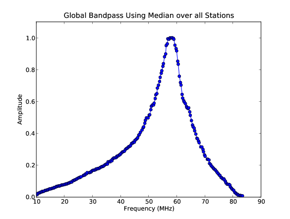
Fig. 24 The global bandpass in LBA between 10–85 MHz.¶

Fig. 24 shows the amplitudes found by BBS for each sub band, normalized to 1.0 near the peak at \(\approx 58\) MHz. The time and elevation evolution of the bandpass has also been investigated. In general, the bandpass is approximately constant on average over the elevation range probed by these observations, implying that the effects of the beam have been properly accounted for.

HBA¶

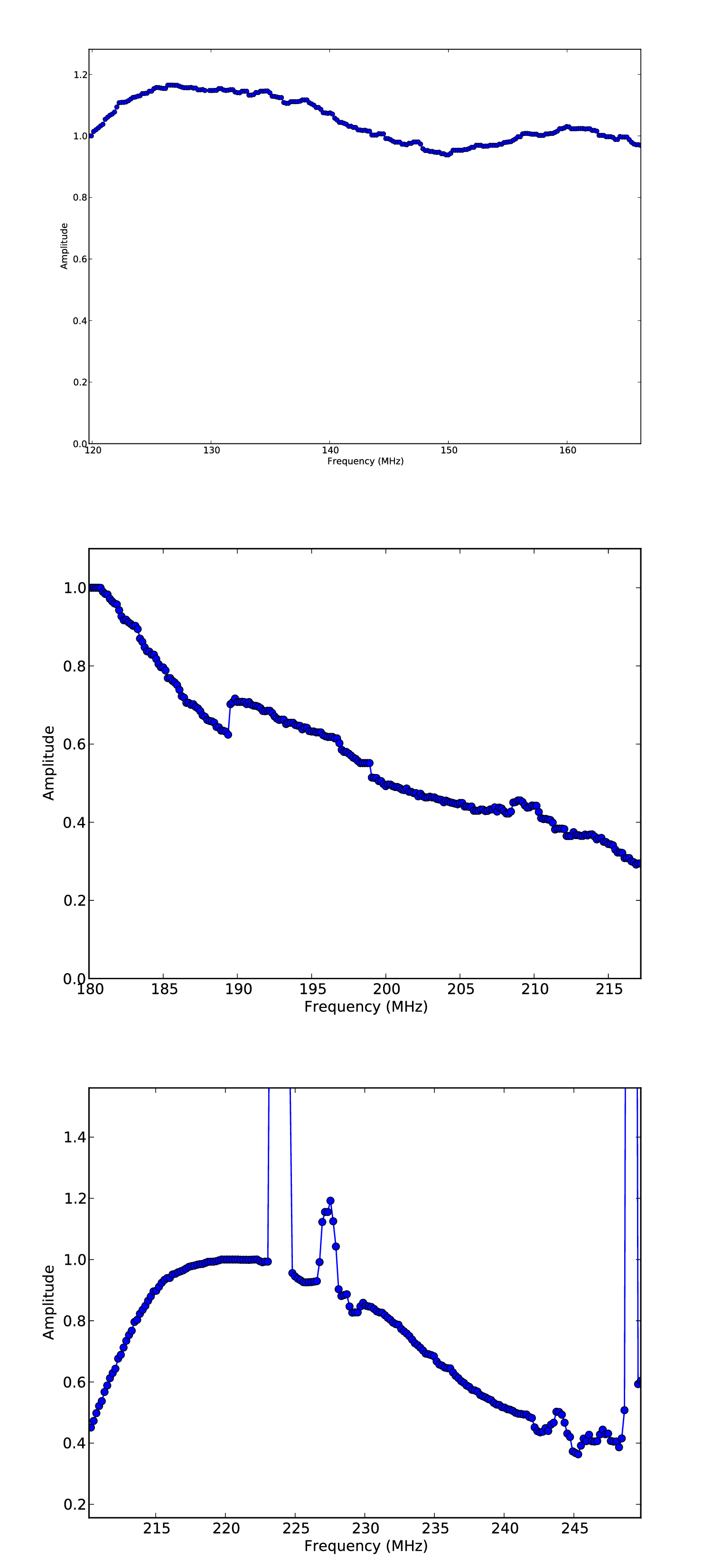
Fig. 25 The global bandpass for the HBA.¶

The global bandpass for the HBA bands was determined in the same basic way as the LBA global bandpass. Three one-hour observations of 3C196 from April 2012 were used (one each for HBA-low, HBA-mid, and HBA-high). No demixing was done. A two-point-source model was used for calibration. The resulting bandpass is shown in Fig. 25. Note that several frequency intervals in the HBA-high observation were affected by severe RFI.

.. _gain transfer:

Gain transfer from a calibrator to the target source¶

In order to calibrate a target field without an a priori model, one way forward is to observe a well-known calibrator source, use it to solve for station gains, and apply those to the target field in order to make a first image and begin self-calibrating. There are two tested methods for utilizing calibrator gains in LOFAR observations. Additional methods may become possible later.

Observe a calibrator source before a target observation, using the same frequency settings, with a short time gap between calibrator and target. This is the same approach as is used in traditional radio telescopes and allows using the full bandwidth in the target observation. However, it is not suggested for long target observations, because the calibrator gains may only remain valid for a relatively short time.
Observe a calibrator in parallel with a target observation, using the same frequency settings for both beams. This has the disadvantage that half of the bandwidth is lost in the target observation, but the time variation of the station gains will be available.

The recommended approach for dealing with both of these cases is outlined below.

The “traditional” approach¶

When doing calibration transfer in the normal way, i.e. the calibrator and target are observed at different times, some work needs to be done before the gain solutions of the calibrator can be transferred to the target. This is because the calibrator solutions tell the gain error of the instrument at the time the calibrator was observed, and in principle not of when the target was observed. The implicit assumption of the traditional approach is that the gain solutions are constant in time. The frequencies of the calibrator observation should in principle match those of the target.

The above means that the calibration of the calibrator should lead to only one solution in time. This can be achieved by setting CellSize.Time to 0. After this is done, the validity of this solution should be extended to infinity by using the export function of parmdbm. Full documentation for that program is available on the LOFAR wiki.

In order to achieve time independence you should use these settings in the BBS parset 16

Strategy.ChunkSize = 0               # Load the entire MS in memory
Step.<name>.Solve.CellSize.Time = 0  # Solution should be constant in time
Step.<name>.Solve.CellChunkSize = 0

Export the calibrator solutions so that they can be applied to target field (see the LOFAR wiki for details). For example:

> parmdbm
Command: open tablename='3c196_1.MS/instrument'
Command: export Gain* tablename='output.table'
Exported record for parameter Gain:0:0:Imag:CS001HBA0
Exported record for parameter Gain:0:0:Imag:CS002HBA0
... more of the same ...
Exported record for parameter Gain:1:1:Real:RS307HBA
Exported record for parameter Gain:1:1:Real:RS503HBA
Exported 104 parms to output.table
Command: exit

An alternative scheme to make the solutions of the calibrator observation time independent is to have a smaller CellSize.Time, and afterwards take the median 17. This way, time cells where calibration failed do not affect the solutions. To follow this scheme, calibrate the calibrator as you would do normally, for example with CellSize.Time=5. To make the solutions time independent, use the tool parmexportcal.py (see parmexportcal –help or its documentation. For example, if you have calibrated the calibrator and stored the solution in cal.parmdb, you can take the median amplitudes as follows

parmexportcal in=cal.parmdb out=cal_timeindependent.parmdb

By default, parmexportcal takes the median amplitude, and the last phase. This is because the phase always varies very fast, and taking the median does not make sense. One can also chose not to transfer the phase solution of the calibrator at all, by setting zerophase to false in parmexportcal.

More advanced schemes for processing calibrator solutions before transferring them to the target can be applied using LoSoTo. An example could be flagging the calibrator solution, and then averaging it (instead of taking the median).

To apply the gain solutions to target field, one can use BBS. For the calibrate-stand-alone script, use the –parmdb option. Use a BBS parset which only includes a CORRECT step. Now you should have a calibrated CORRECTED_DATA column which can be imaged.

The LOFAR multi-beam approach¶

Unlike other radio telescopes, LOFAR has the ability to observe in multiple directions at once. We are currently experimenting with transferring station gains from one field (a calibrator) to a target field. So far it seems to work quite well, with limitations described below. The requirements for this technique are:

The calibrator and target beams should be observed simultaneously, with the same subband frequency. Future work may change this requirement (we may be able to interpolate between calibrator subbands), but for now the same frequencies must be observed in both fields.
Any time and/or frequency averaging performed (before these calibration steps) on one field must be done in exactly the same way for the other field.
The calibrator beam should not be too far from the target beam in angular distance. Little guidance is currently available for the definition of “too far”, but it appears that a distance of 10 degrees is fine at \(\nu\,=\,150\) MHz, while 40 degrees (at the same frequency) might well be too far. Future experiments should clarify this limitation.
In HBA, the distance limit is also driven by the flux density of the calibrator, and the attenuation by the tile beam. For a good solution on the calibrator, ensure that the sensitivity is sufficient to provide at least a signal-to-noise ratio of \(2-3\) per visibility. The tile FWHM sizes and station SEFDs are available online.

In order to do the calibration, and transfer the resulting gains to the target field, follow these steps:

Calibrate the calibrator using BBS. The time and frequency resolution of the solutions can be whatever is needed for the best results. Ensure that the beam is enabled.
```
Step.<name>.Model.Beam.Enable = T
```
(Optional) Perform some corrections to the calibrator solutions, for example flagging, smoothing or interpolation. This is best done in LoSoTo.
Apply the gain solutions to the target field. For the calibrate script, use the –instrument-db option. For the calibrate-stand-alone script, use the –parmdb option. Use a BBS parset which only includes a CORRECT step. Again, ensure that the beam is enabled. The source list for the CORRECT step should be left empty:
```
Step.<name>.Model.Sources = []
```
Before proceeding with imaging and self-calibration, it may be advisable to flag and copy the newly created CORRECTED_DATA column to a new dataset using DPPP.

Post-processing¶

The calibrated data produced by BBS can contain outliers that have to be flagged to produce a decent image. It is recommended to visually inspect the corrected visibilities after calibration. Outliers can be flagged in various ways, for instance using AOFlagger or DPPP.

Troubleshooting¶

Bugs should be reported using the LOFAR issue tracker.
If BBS crashes for any reason, be sure to kill all BBS processes (bbs-controller, bbs-reducer, and bbs-shared-estimator) on all of the nodes you were working on before running again.
After calibrating many frequency channels (e.g. for spectral line imaging purposes), the spectral profile could show an artificial sin-like curve. This is due to the fact that BBS applied a single solution to all the input channels. To avoid this, it is important to set the parameter Step.<name>.Solve.CellSize.Freq to a value higher than 0, indicating the number of channels that BBS will try to find a solution for (0 means one solution for all the channels). You can inspect the solutions with parmdbplot to judge if this is required.
The :math:`<`key name:math:`>`*.log files produced by BBS may provide useful information about what went wrong. Inspect these first when BBS has crashed. The log files from bbs-reducer are usually located on the compute nodes.
BBS expects information about the antenna field layout to be present in the MS. The data writer should take care of including this, but in some cases it can fail due to problems during the observation. The program makebeamtables can be used to manually add the required information to an existing MS. Documentation is available on the LOFAR wiki.

Common problems¶

In the following some error messages are reported together with the solution we have found to fix them.

Station is not a LOFAR station:

Station <name> is not a LOFAR station or the additional information needed to compute the station beam is missing.

Solution: Run makebeamtables on all subbands to add the information required to compute the station beam model.

setupsourcedb failed:

[FAIL] error: setupsourcedb or remote setupsourcedb-part process(es) failed

Solution: Check your source catalog file. You can run makesourcedb locally on your catalog file to get a more detailed error message:

makesourcedb in=<catalog> out="test.sky" format="<"

Database failure:

[FAIL] error: clean database for key default failed

Solution: Check if you can reach the database server on ldb002 and make sure that you created your personal database correctly.

Footnotes

1: This section is maintained by Tammo Jan Dijkema). It was originally written by Joris van Zwieten and Reinout van Weeren.
2: For calibration with DPPP this is not necessary.
3: Examples of these files can be found at https://github.com/lofar-astron/LOFAR-Cookbook <https://github.com/lofar-astron/LOFAR-Cookbook>.
4: Use DPPP’s predict step for this, it is much more efficient.
5: This example can be found at https://github.com/lofar-astron/LOFAR-Cookbook.
6: This example can be found at https://github.com/lofar-astron/LOFAR-Cookbook.
7: This is important when doing a self calibration. In that case only the CORRECTED_DATA column should be used for imaging, while a next calibration step should go back to take the DATA column as input to refine the calibration.
8: This example can be found at https://github.com/lofar-astron/LOFAR-Cookbook.
9: This source catalog is available at https://github.com/lofar-astron/LOFAR-Cookbook.
10: Currently, it is not possible to combine multithreading with a global solve or with the calibrate script.
11: You can copy this file from https://github.com/lofar-astron/LOFAR-Cookbook.
12: Examples can be found in https://github.com/lofar-astron/LOFAR-Cookbook.
13: Actually, both scripts use different terminology, sky-db in the one is called sourcedb in the other. This will be fixed.
14: On CEP3, catalog files with up to ca. 10,000 clean components can be processed until the nodes run out of memory.
15: Available at the LOFAR-Contributions GitHub repository: https://github.com/lofar-astron/LOFAR-Contributions.
16: Note that these settings would be dangerous for a long observation!
17: This is the calibration scheme that the LOFAR pipelines follow.
18: The effect Rotation is stored in the instrument table as RotationAngle.
19: The effect FaradayRotation is stored in the instrument table as RotationMeasure.
20: The effect CommonRotation is stored in the instrument table as CommonRotationAngle.

Calibration with BBS 1¶

Overview¶

Usage¶

Source catalog¶

Gaussian sources¶

Spectral index¶

Rotation measure¶

GSM¶

Special cases¶

Generating a higher resolution skymodel¶

Instrument tables¶

Model¶

Beam model¶

Solver¶

Example reductions¶

Simulation¶

Gain calibration (direction-independent)¶

Gain calibration (direction-dependent) with source subtraction¶

Tweaking BBS to run faster¶

Multithreading¶

Global parameter estimation¶

Setting up your environment¶

Usage¶

Defining a global solve¶

Pre-computed visibilities¶

Inspecting the solutions¶

The global bandpass¶

LBA¶

HBA¶

Gain transfer from a calibrator to the target source¶

The “traditional” approach¶

The LOFAR multi-beam approach¶

Post-processing¶

Troubleshooting¶

Common problems¶

Calibration with BBS 1 ¶