
Introduction
LOFAR
LOFAR (the LOw Frequency ARray) is currently the largest radio telescope operating down to the lowest frequencies that can be observed from Earth. Unlike single-dish telescopes, LOFAR is a large radio interferometric aperture synthesis network of antennas with a computer and network infrastructure that can handle extremely large data volumes.
The operating frequency range of LOFAR is 10 MHz to 240 MHz, while the antennas are optimized for the ranges of 30-80 MHz and 120-240 MHz. These two operating antenna ranges correspond to the Low Band Antenna (LBA) and the High Band Antenna (HBA) respectively. LOFAR antennas are grouped together into 52 stations: there are 38 stations in the Netherlands (24 core and 14 remote stations) and 14 international stations in Germany (6), the UK (1), France (1), Sweden (1), Poland (3), Ireland (1) and Latvia (1). The instrument can be used at an "intermediate" resolution, in which case only the Dutch stations are being used to image at 6" resolution in HBA mode and 15" resolution in LBA mode, or as a VLBI instrument where resolutions down to 0.3" in HBA mode and 0.8" in LBA mode can be achieved using the international stations and a VLBI data processing pipeline.
The LOFAR stations send out various data streams to the central correlator which can output different data products. In what follows, we are going to concern ourselves with (post) processing of visibility (interferometric) data. The visibilities are produced when station data streams are correlated between each pair of stations for every observation (calibrator or target).
In addition, there are various station operating modes and corresponding beams to keep in mind when considering the data reduction strategy. In both LBA and HBA modes, the stations are phased up to form a station beam, where multiple parallel station beams can be formed simultaneously. This allows LOFAR to observe in different directions on the sky at the same time. However, when pointing in different directions in HBA mode, we need to make sure that the pointing centers are not too far apart (certainly not beyond the tile beam which has around 10 degrees FWHM).
Data: format, processing and access
The data format used is the Measurement Set (MS). It is a type of data structure that stores the visibilities and associated metadata in different tables. For more in depth information please refer to the MS data format definition for LOFAR and/or the CASAdocs. The naming convention for each LOFAR measurement set (also referred to as a sub-band) is Laaaaaa_SAPbbb_SBccc_uv.MS, where Laaaaaa is the observation/pipeline SAS ID, SAPbbb is the sub-array pointing (beam), and SBccc is the sub-band (SB) number. A typical observation will (at least) consist of a scientific target as well as calibrator pointing(s). The purpose of the calibrator observation is to use a bright known source to determine the instrumental delay corrections, bandpass, clock offsets as well as some ionospheric corrections. More details about these corrections will be provided in the appropriate sections below.
Due to the requirement that the data can be processed in both medium and high resolution modes, the data streaming from the stations is kept at relatively high resolution, resulting in large (raw) data sizes. In interferometric mode, the time resolution post correlation is usually 1 second, and raw SBs are channelized to 64 ch/SB (192 kHz/SB) although up to 512 ch/SB is possible, but not always feasible. The data size from one observation several hours in duration can easily reach hundreds of TB in size.
The raw and/or processed data are stored on tape storage in the LOFAR Long Term Archive (LTA). Users can request and stage the data for download as well as perform a wide range of data queries. Once the proprietary period expires, the data is public and available for download to every user having an LTA account.
Measurement Sets containing raw visibilities can be processed in several stages using ASTRON's processing pipelines. In data processing order, they are:
- Pre-processing, which allows for RFI flagging as well as time and frequency averaging and compression (employing the Dysco algorithm). This reduces the data size, allowing for more efficient archiving, and conditions the data for further processing. Optionally, the undesired side-lobe signal of extremely bright sources on the sky (the so-called A-Team of Cygnus A, Cassiopeia A, Virgo A and Taurus A) can be removed using the 'demixing' algorithm (mostly relevant for the LBA). This pipeline is usually run on the raw data after each observation before the data is ingested into the LTA by the observatory only.
- LINC (formerly known as Pre-factor) is the direction-independent calibration and imaging pipeline for LOFAR developed and maintained by ASTRON.
- RAPTHOR (the successor of Factor software pipeline) is the direction-dependent calibration and imaging pipeline for LOFAR developed and maintained by ASTRON. It uses the data output by LINC, produces images with a PSF size equal to the synthesized PSF of the Dutch LOFAR array.
- The LOFAR-VLBI pipeline. It uses LINC data output as a starting point to calibrate and image to the maximum LOFAR resolution using the international stations (0.3" PSF size).
The MS format was chosen due to its flexibility and simplicity. Also because of the fact that it is adopted by many different facilities and software tools which are standard for data reduction in radio astronomy e.g. CASA. However, due to the LOFAR data volumes and complexity, as well as the unique calibraton and imaging challenges it entails, dedicated suite of software tools (DP3, AOFlagger, WSClean) and pipelines have been developed to facilitate easier and faster data reduction. These tools are now also widely used for other radio interferometers.
This document focuses on the physical principles underlying the LINC calibration procedure, as well as explaining how to configure and run the pipeline.
RIME
In order to understand some of the terminology of how the pipeline is implemented and the physics involved, it is important to explore the mathematical framework that underlies the pipeline. LINC is based on the Radio Interferometer Measurement Equation: or RIME. In the most basic terms, RIME is a algebraic framework that describes the measured quantity at the output of a receiving element in terms of various instrumental as well as propagation effects that ‘corrupt’ the measurement of the true sky brightness distribution. These effects (assuming linearity) are simply expressed in the form of Jones matrices applied in a specific order (due to the nature of matrices). The most simple form of this is e.g. \bold{\nu} = \left ( \begin{matrix} \nu_a \\ \nu_b \end{matrix} \right )= \bold{J} \bold{e}, where ν and e are column vectors of 2 complex numbers and J is a 2 x 2 complex Jones matrix. There are multiple effects at play before a signal is measured (such as a phase delay, rotations, etc)., then the Jones matrix can be replaced with a so-called Jones chain: \bold{\nu} = \bold{J}_n \bold{J}_{n-1} ...\bold{J}_1 \bold{e}
This form needs to be expanded, as the above equations are only for a single receiver. LOFAR contains many stations that are correlated together and each have their own phase delays, instrumental effects etc. At the same time, the dipoles are not only receiving a single signal, but they observe the entire sky. If we take 2 separated antennas p,q, each measures independent voltage vectors (for each dipole a voltage) \bold{\nu_p}, \bold{\nu_q}, then the fullest yet still intuitive form of RIME is:
| V_{pq} = 2 \left < \bold{\nu}_p \bold{\nu}_q^H \right > = \bold{G}_p \left ( \int_{l} \int_{m} \bold{E}_p B \bold{E}_q e^{-2 \pi (u_{pq}l + v_{pq}m)} dl dm \right ) \bold{G}_q^H |
here, V_{pq} is the visibility matrix output by the correlator for a given baseline defined by these antennas, \bold{B} is the "original" signal brightness and \bold{E} and \bold{G} are part of a Jones chain. From the above equation it is easy to see that \bold{G} is outside of the integral, while \bold{E} is inside. This means that there is a direction-independent (DI) Jones chain (\bold{G}, independent of the directional cosines l m) and a direction-dependent (DD) Jones chain (\bold{E}, dependent on the directional cosines l m).
Intuitively, this equation says that each baseline (comprised by antennas p and q) observes a different visibility ( represented by the visibility matrix), which is a “corrupted” (Jones chain, DI and DD) 2D Fourier transform of the original sky brightness distribution (\bold{B}).
Since LINC deals only with the direction-independent effects, it will thus only solve for the \bold{G}_p and \bold{G}_q matrices for each baseline (which in themselves are a Jones chain, a.k.a. multiple effects G_{p_{1}} G_{p_2} . . . G_{p_n} , G_{q_1}G_{q_2} . . . G_{q_n}), so LINC will consider the following expression:
| V_{pq} = \bold{G}_p X_{pq} \bold{G}_q^H |
where X_{pq} is the 2D Fourier transform of the sky brightness (sometimes called sky coherency). This will serve as the reference equation. As the manual expands on the different sections and steps of LINC the associated matrix in the Jones chain will be presented (where applicable). Note that due to the nature of matrices, the order in which the matrices are applied matters. The following sections will be addressed in reverse order of the signal path (starting at the antenna working back to the sky) which is synonymous to the Jones chain matrix order. For more information about the derivation and RIME expressions, please refer to Smirnov's RIME paper series.
Figure 1: Simple schematic overview of two antennas (p and q) each with two dipoles (x and y) that receive a signal, where one is delayed w.r.t. the other.
The table below gives an overview of the various types of gain matrices
Shape | Calibration type | Free parameters | ||
|---|---|---|---|---|
| fulljones | 8 | ||
| diagonal | 4 | ||
| phaseonly | 2 | ||
| scalarphase | 1 |
LINC
The LINC (LOFAR INitial Calibration pipeline) produces direction-independent calibrated visibilities, a wide-field image of the target field, calibration solutions and diagnostic plots. LINC corrects for various instrumental and ionospheric effects for HBA and LBA observations. The benefit of using LINC over other processing methods (e.g. CASA, AIPS) is that it is largely automated, so it requires little input from the users as well as preparing the data for direction-dependent calibration using dedicated pipelines. For more information about LINC's strategy please refer to the Systematic Effects in LOFAR paper.
To this aim LINC will do the following:
- Remove clock offsets between stations (the LOFAR core stations share a common clock).
- Align the XX and YY polarizations.
- Perform time-independent bandpass correction.
- Correct for ionospheric rotation measure (Faraday rotation).
- Apply the LOFAR beam pattern.
- Perform advanced flagging, mitigate the broad-band RFI and remove bad stations.
- Perform direction-independent phase-only self-calibration on the target data.
- Provide detailed diagnostics of the calibration process.
LINC is composed of two pipelines: the Calibrator Pipeline (CP) & Target Pipeline (TP). The CP processes the calibrator data to derive direction-independent instrumental corrections, while the TP transfers the derived corrections to the target and then performs direction-independent phase self-calibration on the target data, as well as imaging. In order to run LINC the user provides a .json file, containing the path to the data to be processed as well various settings which can be edited to the desired specifications (a more detailed view of the .json specifications can be found here).
In the following sections, the underlying physical principles and algorithms of the data handling by the different pipelines will be presented in short for both the CP and TP. After that, there is a more detailed look into the .json inputs and what steps should be taken in order to customize LINC to a given data set. Finally, the various inspection plots produced by LINC will be discussed and how to interpret them.
Figure 2: General flow of the LINC pipeline, highlighting the important inputs and products.
How to obtain LINC
For users that want to be able to run LINC in their own environment, please refer to the LINC Downloading and installing manual which describes manual and Docker/Singularity installation methods.
Calibrator pipeline
Calibrators are used to correct for instrumental effects and in general set the flux scale for the data: the Calibrator Pipeline aims to do exactly that. This section will step through the workflow of the pipeline and describe what it does, why it does this and how a user should set up a processing run.
Furthermore, the pipeline will also flag 'bad' data. Flagging this "bad data" (RFI, other bright sources that interfere, bad antennas) is important to do before one proceeds with calibration, to ensure that the calibration converges. Due to the nature of interferometry, a malfunctioning antenna or a RFI spike can influence the final image (since the recorded visibilities are Fourier Transformed to the Sky Brightness Distribution).
This section will dive into the physical processes and reasoning behind different corrections that LINC handles. These physical effects are explained and presented using the Radio Interferometer Measurement Equation (RIME) framework that is relevant for LINC's processing.
The process of running LINC is largely automatic where the users has a few responsibilities: setting up the correct control parameters, running the pipeline and inspecting the returned solution plots. A nice overview of what are the necessary and most-common parameters the user needs to adjust can be found on the LINC documentation page. The sections below will elaborate on what LINC does during its run and how to inspect the plots produced in each stage.
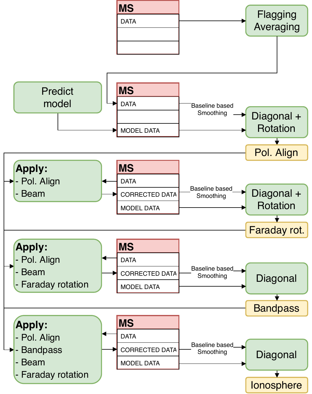
Figure 3: Schematic view of the LINC calibrator workflow and that sections of the measurement set are involved (middle), what steps are applied (left side) and what is derived (right side).
Preparation of the calibrator data
The prep workflow prepares and optimizes the data before the calibration pipeline begins. Mainly it focuses on flagging/removing 'bad' data and averages the input measurement sets (MS) to a more manageable size. Firstly, prep performs RFI flagging with AOflagger, which includes flagging of low-response edge channels, RFI spikes during the observation and more. If necessary, some bright sources will be removed from the data (specifically the A-team sources). Some bright sources in the sky (such as Cyg A) can be detected by LOFAR's station side-lobes and thus can contribute significantly to the image. A sky model of these sources will be used to "demix" these effects. The pipeline will check if there are A-team sources nearby and use a known sky model to account for the side-lobes they can create. It will automatically demix or clip the visibilities depending on the offending source distance from the observation pointing center. This is followed by some averaging that brings the data to a 4 second time resolution and has a 1-to-4-channels per sub-band frequency resolution (depending on the observing mode, LBA or HBA).
Find initial calibrator phase-only solutions using a Skymodel
It is beneficial to incorporate a calibrator sky model into each MS once at the beginning of the pipeline. This is a preliminary known calibrator sky model and is appended to the MODEL_DATA column of the MS and will be used as an initial reference to perform a first phase-only correction. Essentially this will correct the phases to what the source is expected to look like from previous observations to avoid new heavy computations without a model. This will therefore make computations faster for the coming steps.
Correction of Polarisation Misalignment
Some LOFAR stations have a constant time delay between the 2 cross polarizations X and Y, this is what is called polarization misalignment. Unpolarized sources should have a zero difference between the 2 cross polarizations XX and YY. Despite observing known unpolarized sources, LOFAR data does show a polarization misalignment at all frequencies.

Figure 4: XX - YY polarization difference plot. Note how CS013 shows an uncorrected artefact.
This happens because the X and Y polarization data streams are formed independently. Additionally each stream automatically has different station calibration tables applied aiming to compensate for different delays and sensitivity of the individual station dipoles. Usually the polarization offset is constant in time, thus making this effect a phase-only diagonal matrix. However, LINC will solve this as a diagonal plus a rotation Jones matrix. The reason for this combination is to capture some of the 'stray solutions' through the rotation matrix that accounts for some initial Faraday Rotation. The diagonal matrix is dependent on the phase difference, where the X cross-polarization has been set as the reference (hence \bold{J}_{diag}_{11} is 1).
| \bold{J}_{PA} = \bold{J}_{rot} \cdot \bold{J}_{PA \ diag} = \left ( \begin{matrix} cos(\alpha) & sin(\alpha) \\ -sin(\alpha) & cos(\alpha) \end{matrix} \right ) \cdot \begin{pmatrix} 1 & 0\\ 0 & e^{\Delta \phi} \end{pmatrix} |
The polarisation misalignment manifests as a delay between the X and Y data streams, this means the corresponding phase difference has a characteristic frequency dependence \Delta\phi = 2\pi\nu\Delta{t}. This is used in LoSoTo to fit a constant X-Y delay per antenna, strongly reducing the free parameters.
The (Faraday) rotation matrix describes the relationship between the X and Y components of the voltages before and after the rotation. These components change, hence the Faraday rotation affects the amplitudes of the components as well as the phase.
|
Figure 5: Schematic of the mathematical principles of polarisation misalignment being a rotation effect.
The solutions will be derived with the tool LoSoTo, which will also return inspection plots under the directory name inspection/. LoSoTo will return plots for phase (difference) solutions, rotation angle solutions, polarization alignment solutions and more. After solving for this diagonal + rotation matrix, the Polarization Alignment (PA) solutions (the diagonal matrix only) will be applied to the data.
Dipole beam correction
The LOFAR antennas are sensitive to the entire sky due to the construction, this means that the dipoles also observe the entire sky. The so-called dipole beam therefore sees the entire sky. The X and Y dipoles are accounted for by using a 2 x 2 full-Jones matrix:
| \bold{J}_{element \ beam} = \left ( \begin{matrix} a_{xx} e^{i \phi_{xx}} & a_{xy} e^{i \phi_{xy}} \\ a_{yx} e^{i \phi_{yx}} & a_{yy} e^{i \phi_{yy}} \end{matrix} \right ) |
LINC will use a known theoretical dipole-beam model and applies it to the data after the PA correction.
Faraday Rotation
Faraday rotation (FR) is a consequence of the signal propagating through the Earth's ionosphere. The signal travels through a medium that has changes in the index of refraction n, causing the waves to propagate at different speeds, at different angles and at different times, specifically the rotation of the EM field vector. Faraday rotation is a 2nd order frequency correction for this overall phenomenon and depends on the total electron density of the ionosphere and Earth's magnetic field. The observational effect is that the polarisation angle is rotated as a function of frequency, hence it can theoretically be described in terms of a rotation matrix (in linear polarisation basis).
LINC treats this step in the calibration process as a diagonal plus rotation Jones matrix. Here the additional diagonal matrix is there to capture 'leakage' from the beam model imperfections and the bandpass(which will be captured next) to get the best and purest possible rotation matrix.
| \bold{J}_{FR} = \bold{J}_{FR \ rot.} \cdot \bold{J}_{diag} = \left ( \begin{matrix} cos(\alpha) & sin(\alpha) \\ -sin(\alpha) & cos(\alpha) \end{matrix} \right ) \cdot \begin{pmatrix} ae^{i \phi} & 0\\ 0 & ae^{i \phi} \end{pmatrix} |
The LoSoTo tool will be used to derive this correction using the appropriate solution step and will produce new inspection plots. Once the matrix solutions are found, the rotation matrix solutions are used to estimate the time-dependent Faraday rotation by fitting a \nu^{-2} dependency on the solutions. Once this has been found, LINC will apply the PA (diagonal), dipole beam (model) and FR (fitting on rotation) solutions (in that specific order) to the data.
Bandpass Correction
The instrument has a particular response pattern that depends on frequency, in LOFAR this is largely shaped by the dipoles. Some examples of the different effects that create this response pattern are: a) frequency dependency of the dipole beam, b) HBA ripples due to standing waves and c) improper conversion by the poly-phase filter. In order to isolate and ignore time-dependent ionospheric scintillation from these amplitude bandpass corrections, the median of each channel over the entire observation will be taken (making this time-independent and direction-independent) which will be applied to the target fields. The bandpass (BP) solutions should re-scale the flux density of the targets. This effect in LINC is described by a diagonal matrix
| \bold{J}_{bandpass} = \begin{pmatrix} a_{xx} & 0\\ 0 & a_{yy} \end{pmatrix} |
The BP solutions will be derived using LoSoTo with some additional flagging to reject bad solutions and smooth the result. All the previously derived solutions: PA, dipole beam, FR and BP, will be applied to the data.
Clock Drift Correction and Ionospheric Calibration
For LOFAR1, the core stations are all connected to the same GPS-corrected rubidium clock, but remote and international stations have a clock each. These clocks drift around approximately 10 ns per hour to 20 ns per 20 minutes. Although the clocks are periodically re-aligned using GPS signals, there is still an offset as a function of time between the core stations and the other stations. This effect will be described as a scalar when solving for it, since the same clock is used for both polarisations XX and YY. Overall, the clock drift has a time dependence, it can change over the course of an observing run. While solving for the clock drift it will simultaneously also correct for first order ionospheric effects (since the clock drift time is synonymous with a phase delay). So the final phase corrections will be affected by clock (clock) and ionospheric (TEC: "Total Electron Content") delays, both of which show a characteristic frequency dependence of \propto\nu (clock delay) or \propto \nu^{-1} (ionospheric dispersive delay). Using wide-band data, this can be used to disentangle the two delays in LoSoTo. This leads into the Clock-TEC separation method that LINC uses in order to correct the final phases. A theoretical example of what a clock drift specific diagonal Jones matrix looks like is given below:
| \bold{J}_{clock} = e^{2 \pi i \nu t} \begin{pmatrix} 1 & 0\\ 0 & 1 \end{pmatrix} |
All of the found calibration solutions will be stored (in h5parm format) and will be applied to the calibrator data such that the CORRECTED_DATA column is populated with the entire LINC Calibrator Pipeline corrected results (remember due to the nature of matrices, in specific order of PA, dipole beam, FR, BP and Clock-TEC). The stored calibration solutions are important in the next step of LINC: the target pipeline.
Figure 6: Artistic interpretation of the different physical effects and where they occur along the signal path.
Target Pipeline
The target (or sometimes called the science target) pipeline (TP) in LINC will transfer the previously found solutions from the calibrator pipeline, and perform an initial direction-independent self-calibration on the target. In this section, the LINC pipeline steps for the target pipeline will be described, the produced inspection plots will be shown as well as explained what the user can do with the final diagnostics and images that are produced.
Similarly to the CP, the TP is largely automatic and thus the users have the same few responsibilities: setting up the processing parameters, running the pipeline and inspecting the returned solution plots. A nice overview of what necessary and most-common parameters the user needs to adjust on the corresponding LINC documentation page.
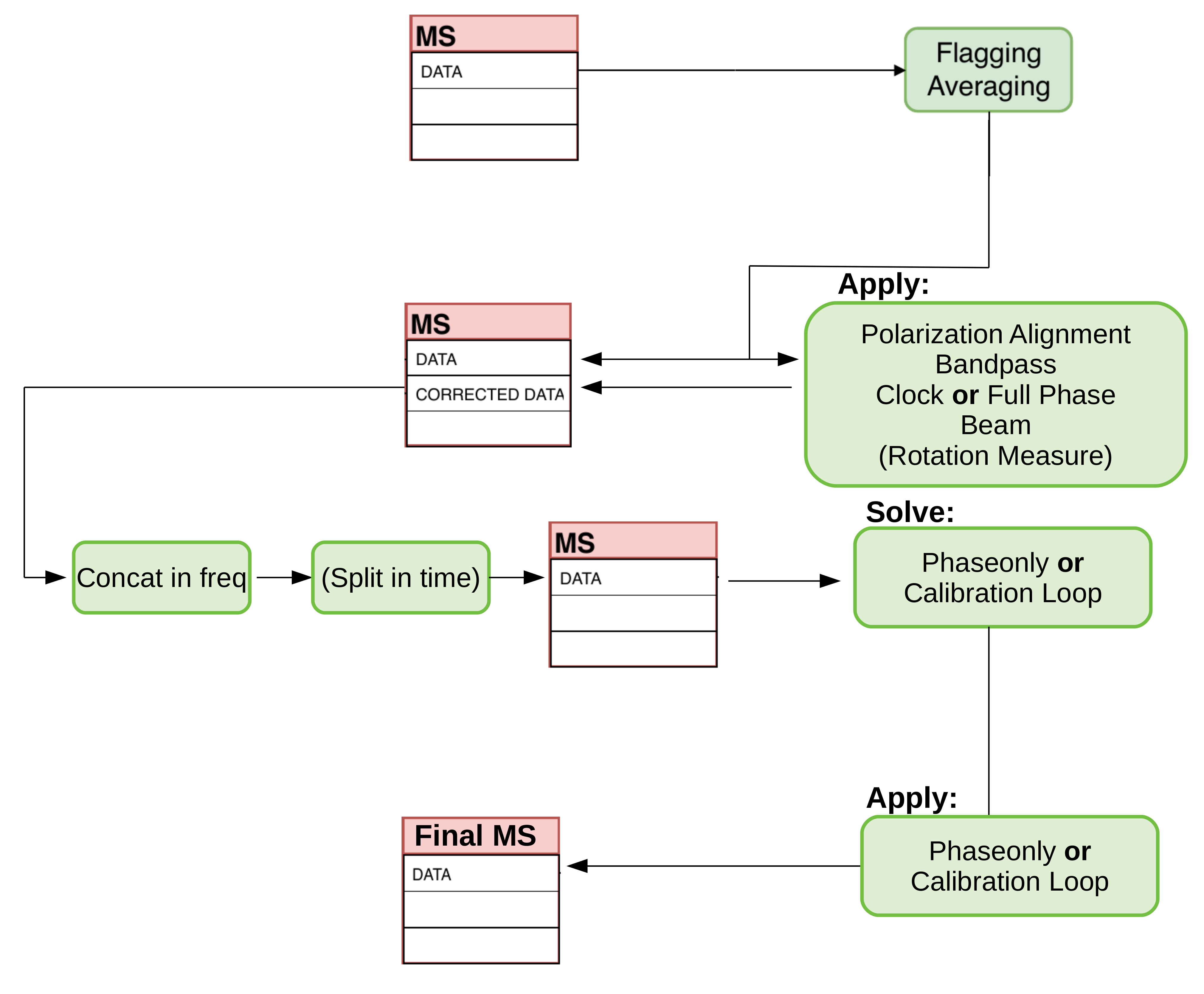
Figure 7: Schematic view of the LINC target workflow and that sections of the measurement set are involved (middle), what steps are applied (green).
Transfer and apply Calibrator Solutions
The previously found calibrator solutions are now used as well in the target pipeline. Meaning that before the target pipeline will derive solutions for the target specifically, it will apply the solutions stored in the h5parm files to the target data. The user will have to specify where the h5parm files are stored (cal_solutions parameter in the .json file) in the input .json file.
Preparation of the target (prep)
Similar to the preparation of the calibrator, the prep workflow will prepare the data before other calibration processes begin. Some of the things that are included in this workflow are:
- check station mismatch between calibrator and target
- demix bright and nearby A-team sources
- basic flagging
- averaging
Phase-only calibration (gsmcal)
The gsmcal workflow aims to derive a first phase calibration w.r.t. the phase centre of the image. The workflow will create a global sky model and calibrate against that. The phases will be calibrated to match the global sky model in order to get a better phase alignment. These phase solutions will be loaded into LoSoTo which will create diagnostic plots for solution inspection.
Final results & useful diagnostics
The final step of the LINC pipeline is to finalise the output and products produced by the workflows. This includes applying the derived solutions to the target, imaging the target using the fast imager WSclean, and some final useful diagnostic plots/files. These plots include: a summary file (containing, for example, percentage of unflagged data), an uv-coverage plot, and the final FITS image made by WSclean.
Configuring LINC
Most of the LOFAR MS's can be processed with LINC's default parameters. The configuration file can be specified and adjusted to the selected data that has to be processed. It is important to know that if, for example, a data set from the LTA is pre-processed and demixed. In this section, the most important parameters for the LINC configuration will be given. For more specific details on how to adjust the .json see this page, plus other important parameters for the CP and TP. Parameters you must define for LINC are:
msindefines the input data (the .ms sets downloaded from the LTA)cal_solutionsdefines the input calibration solutions from the calibrator pipeline that is used for the target pipeline
Some parameters that may need to be adjusted are:
refantsets the antenna the phases will be calibrated in reference to (a.k.a. the antenna that has phase = 0)rfistrategydefines the data flagging strategy, can be set for HBA and LBA separatelyraw_dataset to True if the input data is raw, set to False if the data is pre-processeddemixset to True if demixing should be performed. Recommended to enable for LBA target observations if demixing was not performed by the pre-processing pipeline.
If the default settings do not work for the chosen observation, the user is unsure how to approach the different settings, it is recommended to contact the SDC Helpdesk.
Interpreting Inspection Plots and Diagnostics
It is important to check what the produced inspection plots spit out after running the pipeline to see if it found good solutions and that they are sensible, and if not interject and process the failures manually. This section will provide some general plots to look out for that are produced by LINC and what to look for within them.
Calibrator Pipeline Products
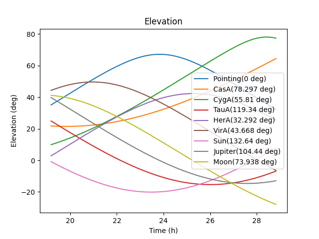
The Ateam_separation plot shows the A-team source elevation across the observation and (if 'demix' was set to True) it can be used to see if the removal of a (or more) A-team source(s) was appropriate. If in hindsight, an A-team source was >40 degrees elevation across the calibrator observation, then it is recommended to demix this source (for HBA, for LBA it is always recommended to demix).
The derived bandpass for all stations (shown is bandpass_time<xxx>_polXX.png and bandpass_time<xxx>.png) for HBA should have the same overall shape as the known bandpass, If there are extreme spikes in the bandpass solutions that breaks the continuity of the rest of the bandpass curve, then some flagging might have gone wrong. The right image shows an easier way to identify potential problematic or unresponsive stations.


The fr.png and tec.png are closely related. The fr.png plot shows the differential of the rotation measure (dRM), while the tec.png shows the differential electron content (dTEC). Previously it was mentioned that both the FR and TEC are 2nd and 1st order frequency effects of the ionosphere (respectively). This can be seen back in the plots for the solutions: the tec.png plot tries to capture the strays from the fr.png corrections. For both the plots, for the core stations it should be (close to) 0 and they should vary smoothly. The remote stations and international stations might deviate from the core stations, but as long as they vary smoothly and are not too far off 0 then the solutions are good.


For the clock.png plot it is expected that the core stations (that are tied to the same clock) should exhibit variations or offsets within 10 ns over a day, while remote stations can have variations or offsets within a few tens of ns and the international stations can exhibits 100 ns variations or offsets. If the plots show something wildly different, then something is wrong.

Lastly, it is useful to check the log and summary of the calibration solutions to inspect the percentage of flagged data in the different calibration steps. If there are some large percentages of flagged data, then it is good practice to go back inspecting the solutions and see if something went wrong (e.g. with flagging).

Target Pipeline Products
The Ateam_separation plot shows the A-team source elevation across the observation which is useful for checking the distance of the offending sources w.r.t the observed target. Additionally the Ateam_clipper plot is especially useful to see how much data is clipped/flagged because of the selected close-by A-team sources. The amounts of clipped visibilities depends on the specific sky configurations but typically values <10% are reasonable. Larger values are suspicious that the amount of interference must be treated via the demix, i.e. source removal.

It is important to inspect the ph_polXX.png plot and ph_poldif.png (for the target specifically) to check on the phase solutions. The phase solutions for the core stations should be stable, a.k.a. single colour across the plot. In the plot below this is not the case, where it is due to ionospheric conditions. But in general the core stations should be fairly uniform. For the remote stations this should be similar, the colour should be relatively uniform, possibly with some minor deviations. In the figure below this is not the case, it looks not stable or uniform (again due to the ionospheric conditions of this observation). The remote stations can look like the phases are wrapping, it should be continuous. In the example plot there is some wrapping of phases visible on the remote stations, which is OK. However if it looks completely random then this has to be revisited. Another useful plot is the *dif.png plot, which shows the difference between the polarisations and if ultimately the polarisation alignment was successful. In the example plot, it is rather noisy, preferably these plots should be (largely) uni-coloured.

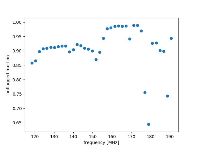
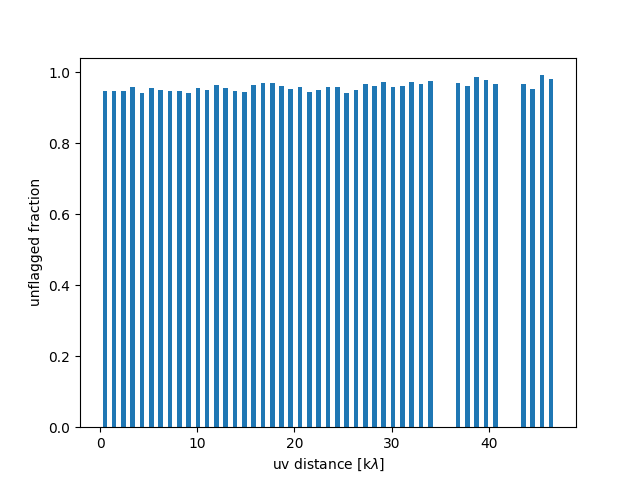
It is recommended to check the log, the unflagged_fraction.png, and the uv-coverage_uvdist.png plots. The summary log returns (amongst other things) the amount of flagged solutions at different stages of the pipeline. This will give a nice first indication that not too much data has been flagged in the process. The unflagged_fraction plot shows, as a function of frequency, how much data remains after all the flagging; this can guide the user to chose the portion of the bandwidth to be further processed and thus ignore bad subbands. In the example plot, it can be seen that mostly >90% of the data remains for certain frequencies, but that frequency ~180 MHz was quite problematic and hence was flagged more (approx 65% of data remains). The uv-coverage_uvdist plot is a nice way to see how much data is left after the processing and thus what the UV coverage is after all flagging: this is relevant depending on the sensitivity needed at specific angular scales the user needs for the target(s). In the example plot most of the data remains unflagged (most uvdist still have >90% of the data left). If any of the flagged percentage of data is very high, it can have drastic consequences on the data so it is wise to keep an eye on these numbers and if need be adjust the pipeline or consider manual processing. A plot for the overall uv-coverage across the entire observation can be viewed in the uv-coverage.png plot. Flagging percentages can also be found in the logs and in the solution summaries.
Lastly, it is important to inspect the final FITS image that is produced in the pipeline. It is useful to note however if the imaged target field is sensible and if there aren't too obvious ripples left in the image that disturb the objects in the target field. Linear ripples (straight lines originating from the bright source) indicate amplitude errors, which was not self-calibrated for and the user can consult another pipeline/program to correct for the amplitude effects. Other forms of ripples could be due to phase errors (could be due to a complex ionosphere, or bad calibration), improper removal of distant disturbing sources or deconvolution artefacts. In the case of the latter, it is wise to consider either different WSClean parameters or manual cleaning.The presence of very strong ripples could also indicate leftover RFI or some failure in the calibration. Some typical noise levels for LBA are approximately 10mJy/beam and for HBA 0.1~0.15 mJy/beam, this can be used to crosscheck if their FITS image has similar levels of noise.
]
Hands-on approach
Aside from LINC, the user can use the LINC calibrated data for manual (offline) reduction, or use helper scripts to gain more insight into the data. Below we show some examples.
- Determining the distance of A-team source(s) from the pointing direction
As described in the Interpreting Inspection Plots section, the Ateam_separation plot can give great insight in what A-team sources should be removed, which can be specified in the .json before running LINC. However, in order to get this plot before running LINC, the user can use the following: plot_Ateam_elevation.py Lxxx_SAPxxx_SBxxx.ms. In this plot, for HBA observations if there are A-team sourced >40 degrees elevation during the observation, then it is wise to demix them.
- Re-imaging of the calibrated data
In the final step of the pipeline, LINC images the calibrated (and averaged) data using the WSClean imager with the following command:
wsclean -auto-threshold 5 -channels-out 7 -deconvolution-channels 3 -fit-spectral-pol 3 -name <target name> -scale 15asec -size 2500 2500 -join-channels -maxuvw-m 20000 -mgain 0.8 -no-update-model-required -multiscale -niter 10000 -nmiter 5 -parallel-deconvolution 1500 -parallel-reordering 4 -taper-gaussian 40asec -temp-dir <temporary file directory> -use-wgridder -weight briggs -0.5 <location of .ms>
Users can re-image the calibrated data by, for example, tapering the visibilities with a 80 arcsec Gaussian taper using an adjusted version of the above command and the calibrated data set (located in the pipeline results directory) as input.The main use of this is to, for example, change the weighting to reveal certain structures (e.g. accentuate diffuse emission or provide easier flux measure of emission).
What follows is a short explanation for each of the parameters in the WSClean command and how to change them.
- auto-threshold → an automatic threshold that is defined relative to the residual noise level (<nr> times the standard deviation of the noise in the image) that ensures cleaning stops at an appropriate level. Normal values are usually between 3-5 (the lower the number the "deeper" the iterations).
- channels-out, deconvolution-channel, fit-spectral-pol, join-channels → these parameters are all related to multi-frequency/wideband deconvolution. The settings allow for combining a deep clean on the image field while incorporating a frequency dependency.
- name → name of the image, has to be unique (it won't be overwritten)
- scale → pixel size pre-determined by the observational set-up (resolution). For Nyquist sampling, the minor axis of the synthesized beam should be at least three pixels across.
- size → Size of the image in pixels (x times y).
- maxuvw-m → sets a maximum baseline length cut (in meters).
- mgain → sets is major iteration gain that reduced the peak by the given factor. This is usually 0.8, but if the psf is good 0.9 could work and can speed up the imaging. If the psf is bad this value can be lowered.
- no-update-model-required → makes sure the model is not appended to the measurement set (if this is desired then it can be removed).
- multiscale → perform cleaning on different scales; especially useful for resolved sources. Please refer to Multiscale Cleaning for further details.
- niter → number of iterations, that is set to a very large number (since the auto threshold will halt cleaning automatically, so niter has to be large to not interrupt the cleaning)
- nmiter → defined the maximum number of major iterations (set to 5 major iterations, can be changed).
- parallel-deconvolution → initiates parallel deconvolution that will start separate deconvolution of the sub-images which helps speed especially for large images. For large images the usual value is between 1024-4096.
- parallel-reordering → if the MSs to be images are (to be) reordered, use multiple threads for the reordering.
- taper-gaussian → tapering is used to shape the synthesised beam which tapers the weight of visibilities in the uv plane. This options is specific for the Gaussian taper which makes the synthesised beam approach a Gaussian function. This can be changed by the user to define a larger synthesised beam size. To see more details on other kinds of tapering see Tapering.
- temp-dir → Define the temporary directory that can be used if memory is an issue.
- use-wgridder → enables the wide-field gridding algorithm that adds a w-direction to uv-gridding where each visibility is gridded to a small range of w-planes
- weight → defines how the flux assigned to each pixel is weighted, which can ultimately reveal different kinds of structures (for example accentuate diffuse emission). The standard is minus 0.5 Briggs weighting but some of the most common ones are: Briggs -2 to 2, natural and uniform weighting. For more detailed information about the weight options are given in Image Weighting.
- Further reading
The LOFAR imaging cookbook contains manual reduction recipes which can still be useful, for example:
Spectral index, Polarization and global sky model