

- in query form say we use the default but more can be found using the service info and topcat/pyvo.
Introduction
The science-ready data products as described in Available data products are exposed through standard Virtual Observatory protocols to facilitate their access and exploration.
The LoTSS DR2 data is hosted on the SURF Data Repository (sdr) system. We recommend astronomers to use the VO interfaces described below for data discovery. Some of the data is stored on tape. This is indicated in the data description in the DataLink document that is returned by the VO query. To access files on tape, users need to obtain an account which gives them the possibility to "stage" the data from the tape to a disk from which it can be downloaded. Data that is stored on disk is directly accessible through the VO.
In particular, the protocols offered are the Tabular Access Protocol (TAP), Simple Application Messaging Protocol (SAMP) and the Simple Image Access protocol (SIA). TAP and SAMP enables queries to explore the data in a tabular form using tools such as TOPCAT. TOPCAT is an interactive graphical viewer and editor for tabular data, it enables the interactive exploration of large tables performing several types of plotting, statistics, editing and visualization of tables. SIA enables the rapid display of images and cubes through all sky atlas tools such as ALADIN. ALADIN is an interactive sky atlas allowing the user to visualize digitized astronomical images/cubes and superimpose entries from astronomical catalogues or databases.
The data published in the VO can also be accessed using a web browser at https://vo.astron.nl. This web interface provides a page on which all the collections present in the registry are listed, including the published LoTSS DR2 data sets:
| Service name | Service Description | Type | Link to column descriptions |
|---|---|---|---|
LoTSS-DR2 Gaussian catalog cone search | catalog | info | |
| LoTSS-DR2 Source catalog cone search | |||
| LoTSS-DR2 mosaics | image |
Selecting a data collection allows the user to perform a cone search through a webform (Fig. 40). The result is either a source or Gaussian list, or a table of data products of that given class overlapping a given pointing. The size of the continuum images as well as the cubes extend beyond the 10% primary beam level for cleaning the secondary lobes of bright offset sources. To ensure that the search is done in the area of maximum sensitivity the search is performed on a maxim radius of 0.75 degrees from the center (this represents the average value of where the sensitivity drops). This value can be modified using the Max distance from center. A different output with respect to the default can be customized using More output fields selection button.
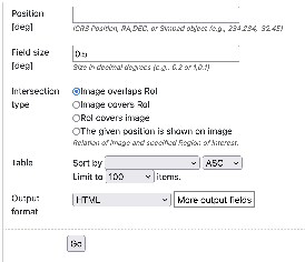
Fig. 40 Query search form for continuum images.
The result is a table in the requested output format in which every row corresponds to a data product (Fig. 41).
In each row there is a column, Product key, which is a link that allows the user to download the fits file of the image of interest. The column titles should generally be self-descriptive. However, the long human-readable description of the content of each column is a tooltip that will appear when hovering over the column name.
The selected target and the position of the individual pointings can be visualized using the Quick plot button at the top of the window of the results of the search query (Fig. 41).
In the column Related products another link connects to a page containing a list of links to additional related data that can be useful to interpret or reanalyze that given product, for which a preview is provided (Fig. 42).

Fig. 41 Result of an image search query. Click for a bigger image.

Fig. 42 Links to data products related to the target of interest. The top two items represent the primary data product (ie the one that can be directly downloaded from the table view) and a link to the thumbnail of that data product. The other products are the anciliary data. Click for a bigger image. Note that the number of related products is too long to fit readably in a single screen shot.
Some data products are directly accessible, in which case the link on this table will initiate a direct download. However, the larger (and rawer) data products are stored on tape (in which case the text 'on tape' appears in the description). The link will then bring you to the entry of the corresponding pointing in the SURF Data repository (Fig. 43/1). If data is on tape, the status is either "online", in which case it can be downloaded by pressing the "Download" button, or "offline" in which case it can be requested to be put online by pressing the "Request" button. Please note that you need to be logged in to perform the request. If a request has been correctly performed, the status of the file will change to "staging" unill it becomes "online".

Fig. 43/1 Surf Data Repository view of the data from a pointing. Click for a bigger image.
The source and Gaussian cone search forms each return a table with source positions and properties. As before, the long descriptions are available using tool tips. The columns "Mosaic_URL" links to the anciliary data product page of the mosaic from where the Gaussian or source was extracted (like e.g. Fig 42).
The columns shown in Figure 41 are the most informative for the astronomers (e.g. position, observing frequency, observing date, quality assessment, format etc), please note that more columns are available but not displayed here. The complete set of columns can be visualized via topcat as described below or using More output fields selection button in the search query. Querying the released data is also possible using e.g. TOPCAT using TAP. Via the TAP protocol, it is possible to query the registry in a more flexible way using an enriched SQL syntax called ADQL. An example is given in Fig. 43 : click the link indicated with the red ellipse on the left panel Try ADQL and place your ADQL query on the query form.
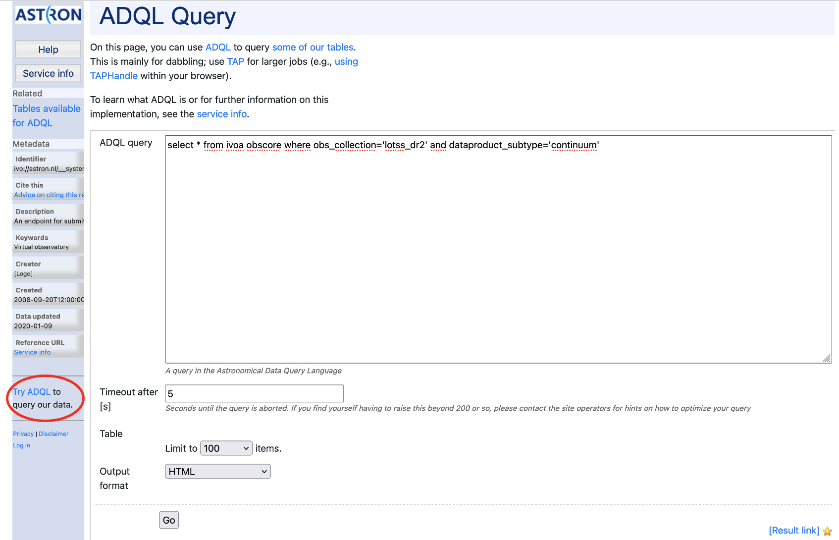
Fig. 43/2 ADQL query form.
The table names to use in the query form of Fig. 43/2, are summarized in Table 10. The URL for the query is then: https://vo.astron.nl/lotss_dr2/q/{Table name}/form (e.g. https://vo.astron.nl/lotss_dr2/q/src_cone/form}.
It is possible to query all the available dataproducts at once by using the table ivoa.obscore and by appending to the ADQL statement “where obs_collection=” it is possible to limit the search to the apertif_dr1 only.
VO-Apertif DR1 Processed Data Products
Table names to be used in the ADQL query.
Table name | obscore type | obscore subtype |
|---|---|---|
gauss_cone | table (not an obscore type) | |
src_cone | table (not an obscore type) | |
lotss_dr2_mosaic | image | total intensity map |
Access via TOPCAT
The Apertif DR1 data collection tables can be accessed using TOPCAT, an interactive graphical viewer and editor for tabular data. The data can be sent from vo.astron.nl to TOPCAT using one of the two protocols: SAMP or TAP. The two subsections below provide a description on how to access the tabular data using either SAMP(link to Send via SAMP subsection) or TAP(link to VO Table Access Protocol (TAP) subsection).
Send via SAMP
With TOPCAT opened, and once you are satisfied with the output of the cone search in the Astron VO webform, click the grey button “Send via SAMP” as shown on the top of the output list of Figure 3. Authorize the connection and wait until the download is completed.
Once completed, the catalogue will be visible in the left panel of TOPCAT (Table List). Click on the new entry as shown by the arrow in Fig. 44. At this point the table browser will open showing the content of the DACHS results (PLACE HOLDER use DR1 in selection). From here any TOPCAT tool can be used for further inspection and analysis of the results. Alternatively the table can be saved in various formats and used locally with other programs (e.g. python scripts etc).
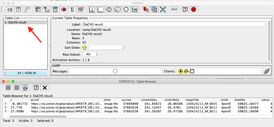
Fig. 44 TOPCAT table browser view of the Apertif DR1 data collection tables. Click for a bigger image.
VO Table Acess Protocol (TAP)
From the TOPCAT menu bar, select VO and in the drop down, select Table Access Protocol (TAP) as shown by the red arrow in Fig. 45.
This will open the Table Access Query window where the ASTRON VO TAP server is listed. Select it and click on Use Service at the bottom of the window (Fig. 46). Another tab will open showing the Apertif DR1 data collection. Select one, e.g. continuum image, and enter a query command in the bottom panel, an example of which is indicated by the red arrow in Fig. 47. Submit the query using Run Query. This will show the resulting table in the Table list view shown before in Fig. 44. From here, any TOPCAT tool can again be used. As mentioned in the previous section, the query result in vo.astron.nl will display a subset of the columns of the Apertif DR1 table (e.g. position, observing frequency, observing date, quality assessment, format etc). The complete set of columns (e.g. pipeline version, wcs references etc) belonging to each data collection of the Apertif DR1 can be explored using the option described in this section.
The position of the targets can be visualized using the option skyplot in TOPCAT, once the search query has been sent via SAMP or TAP as described in this section.

Fig. 45 TOPCAT menu bar for VO services. Click for a bigger image.

Fig. 46 TOPCAT TAP service query form. Click for a bigger image.

Fig. 47 TOPCAT menu bar for VO services. Click for a bigger image.
Another useful way to inspect the Apertif DR1 data collection, but also other data collections exposed via the ASTRON-VO, is the ivoa-obscore table. The same selection as before can be used (Fig. 47) but instead of selecting Apertif_dr1 tables, the table ivoa.obscore is to be selected. In this way it is possible to glance over all the data collections exposed via the ASTRON-VO. This might be useful for instance to enable multi-wavelength science exploring LOTSS and Apertif DR1 data or, as mentioned in the case of the ADQL query, to visualize multiple data collections at once.
Having ALADIN open, and once you are satisfied with the resulting table, it can be sent to ALADIN following the instructions of Fig. 48.
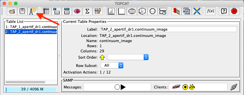
Fig. 48 How to transfer the TOPCAT query results to ALADIN. Click for a bigger image.
Access via ALADIN
Catalogues
The Apertif DR1 VO data collection can also be discovered directly via ALADIN either via simple image access protocol (SIAP) or tabular access protocol (TAP). The examples shown here require the desktop version of ALADIN.
Open ALADIN and on the left panel for SIAP: select Others > SIA2 > astron.nl > The VO @ASTRON SIAP Version 2. Alternatively for TAP select Others > TAP > astron.nl > The VO @ASTRON TAP service (Fig. 49). A pop-up window will open. Click load, and enter a query using the Server selector (Fig. 50) or TAP access with astron.nl/tap (Fig. 51) to select the target of interest for SIAP and TAP respectively.

Fig. 49 ALADIN display panel. Click for a bigger image.

Fig. 50 ALADIN server selector panel for SIAP. Click for a bigger image.

Fig. 51 ALADIN TAP access panel. Click for a bigger image.
After loading, the data collection catalogues can be plotted on the main panel by selecting them first on the right panel (e.g. highlighted in blue in Figures 14 and 15) and then by selecting the regions of interest on the bottom panel as shown in Figures 14 and 15. From here the usual functionality of ALADIN can be used.
HiPS

Fig. 52 Example of data collection selection via SIAP in ALADIN. Click for a bigger image.

Fig. 53 Example of data collection selection via TAP in ALADIN. Click for a bigger image.
Images
Downloading images or cubes in ALADIN is also possible (see Fig. 54). The user will need to click on the url-link in the column access_url of the bottom panel. Then, once the image is loaded, click on the right panel as shown in Fig. 54. From here the usual functionality of ALADIN can be used.

Fig. 54 Example of image selected from the Apertif DR1 displayed in ALADIN. Click for a bigger image.
Python access
The data collection and the table content can be accessed directly via python using the pyvo tool. Working directly in python the tables and the data products can be simply queried and outputs can be customized according to the user’s needs, without the involvement of TOPCAT or ALADIN.
An example of a TAP query and image download can be found in the python script below (it has been tested for python 3.7). The result of the query can also be plotted using python.
#To start you have to import the library pyvo (it is also possible to use astroquery if you want)
import pyvo

## To perform a TAP query you have to connect to the service first
tap_service = pyvo.dal.TAPService('https://vo.astron.nl/__system__/tap/run/tap')

# This works also for
form pyvo.registry.regtap import ivoid2service
vo_tap_service = ivoid2service('ivo://astron.nl/tap')[0]

# The TAPService object provides some introspection that allow you to check the various tables and their
# description for example to print the available tables you can execute
print('Tables present on http://vo.astron.nl')
for table in tap_service.tables:
 print(table.name)
print('-' * 10 + '\n' * 3)

# or get the column names
print('Available columns in apertif_dr1.continuum_images')
print(tap_service.tables['apertif_dr1.continuum_images'].columns)
print('-' * 10 + '\n' * 3)

## You can obviously perform tap queries accross the whole tap service as an example a cone search
print('Performing TAP query')
result = tap_service.search(
 "SELECT TOP 5 target, beam_number, accref, centeralpha, centerdelta, obsid, DISTANCE(" \
     "POINT('ICRS', centeralpha, centerdelta),"\
     "POINT('ICRS', 208.36, 52.36)) AS dist"\
 " FROM apertif_dr1.continuum_images"  \
 " WHERE 1=CONTAINS("
 "    POINT('ICRS', centeralpha, centerdelta),"\
 "    CIRCLE('ICRS', 208.36, 52.36, 0.08333333)) "\
 " ORDER BY dist ASC"
 )
print(result)

# The result can also be obtained as an astropy table
astropy_table = result.to_table()
print('-' * 10 + '\n' * 3)

## You can also download and plot the image
import astropy.io.fits as fits
from astropy.wcs import WCS
import matplotlib.pyplot as plt
import requests, os
import numpy as np

# DOWNLOAD only the first result
#
print('Downloading only the first result')
file_name = '{}_{}_{}.fits'.format(
 result[0]['obsid'].decode(),
 result[0]['target'].decode(),
 result[0]['beam_number'])
path = os.path.join(os.getcwd(), file_name)
http_result = requests.get(result[0]['accref'].decode())
print('Downloading file in', path)
with open(file_name, 'wb') as fout:
 for content in http_result.iter_content():
     fout.write(content)
hdu = fits.open(file_name)[0]
wcs = WCS(hdu.header)
# dropping unnecessary axes
wcs = wcs.dropaxis(2).dropaxis(2)
plt.subplot(projection=wcs)
plt.imshow(hdu.data[0, 0, :, :], vmax=0.0005)
plt.xlabel('RA')
plt.ylabel('DEC')
plt.show()
Export machine readable table
There are multiple ways to export a catalog of the various data products of the data release. On the vo.astron.nl pages, the results of a query can be exported to a csv file or fits table; running an empty query with a table limit of 5000 or more will return all entries.
TOPCAT and the pyvo interface demonstrated above also provide functionality for exporting machine-readable files.
The ADQL form is another option, and below we provide an example query that also provides information about the calibrators used for each beam. This query is specific to the continuum_images data product but can be adapted to other (beam-based, processed) data products by replacing the table name, e.g., for polarization cubes/images use pol_cubes (see Table 10 for a full list of the available tables).
select data.*,
flux_cal.obsid as flux_calibrator_obs_id,
pol_cal.obsid as pol_calibrator_obs_id  from apertif_dr1.continuum_images data
join  apertif_dr1.flux_cal_visibilities flux_cal on data.obsid=flux_cal.used_for and data.beam_number=flux_cal.beam
join apertif_dr1.pol_cal_visibilities pol_cal on data.obsid=pol_cal.used_for and data.beam_number=pol_cal.beam
order by obsid
Overview
Content Tools
Tasks