

Introduction
This page describes access to the data in ASTRON's data holdings using the Virtual Observatory standards. Those standards support access to data like catalogs and images. We introduce the most important standards on this page and give some usage examples tailored to the ASTRON data holdings. If you want more advanced information on how to use the VO standards, you can start with the IVOA website for astronomers and the IVOA wiki page on educational resources. For our data holdings we use the DAta Center Helper Suite (DACHS), which offers a web interface of its own. We will link to several places in DACHS in the documentation but in principle all information showed by DACHS can also be accessed using any VO tools.
Data access protocols
The VO consists of several different protocols. In this section, we describe the important protocols, and provide the acronyms that are generally used in the VO tooling. Most data in vo.astron.nl consist of tables, that can be accessed using the Tabular Access Protocol (TAP). Images are offered using the Simple Image Access Protocol (SIA) which in essence is a table with a field containing a link to an image. A few services offer cutout functionality (using SODA). A cutout is essentially a service that returns an image (or more generally a data product) that only contains the data inside the cone that has been requested by the user.
In some cases, the table describing the data will contain a so-called DataLink document that links the primary data product (often an image or cube) to related data products (e.g. raw visibilities, calibration solutions).
Another relevant VO standard to mention here is the Simple Application Messaging Protocol (SAMP). This protocol makes it possible for applications to share information. This allows users to for example query the VO with one application, visuaklise the results with another and do analysis with a third one.
HiPS
The Hierarchical Progressive Survey (HiPS) protocol defines a way to visualise sky surveys by breaking them up in different hierarchical views which represents different zoom levels. This makes it possible to scroll through a survey in a way that is comparable to using Google Maps (or other online mapping/satellite tools). ASTRONs HiPS collections are all available in Aladin and the most important ones are available through other tools, like ESASky. However users can also have direct access to all our HiPS collections through hips.astron.nl. Typically, HiPS projections are used to visually look through the data from a survey, and combine the coordinates with table-based services to obtain source information or data. The following table shows an overview of the ASTRON HiPS server contains the following data collections.
| Collection name (and link) | Description | promoted |
|---|---|---|
| TGSS ADR | Yes | |
| Apertif DR1 | Apertif first Data Release (DR1) - Uncalibrated continuum flux | Yes |
| LoTSS DR1 low | Lofar Two-Metre Sky Survey (LoTSS) first data release (DR1) low resolution (20") | No |
| LoTSS DR1 high | Lofar Two-Metre Sky Survey (LoTSS) first data release (DR1) high resolution (6") | Yes |
The ObsCore table
One of the tables in vo.astron.nl is called ivoa.obscore . This table is a special table which follows the ObsCore standard defined by the IVOA and it contains key observational information describing all the data products (images, cubes, etc) in our VO service. Currently, there is not service to directly query this table, but it can be done using ADQL.
List of vo.astron.nl services
The data published in the VO can also be accessed using a web browser at https://vo.astron.nl. The web interface can be used to perform simple queries. The power of the VO lies in the fact that several applications exist that can interact with the standards we offer. In the architecture, there is a distinction between services and tables. A service is an entity that takes user input and provides a table as output. The tables themselves are the entities that actually hold the data. Tables can also be queried directly, for instance using ADQL. In the following table, we list the services for accessing data collections in the ASTRON VO. The columns of the table are:
Service name | The (human-readable) name of the service |
| Type | The type of this service. Services of type system are not coupled to specific data collections. The services that provide access to data are either of type image or cube. The image cutout services also offer images, but those are cutouts as define above. Finally there are catalogues which are either catalogues of astrophysical objects, or catalogues which tabulate the properties of the raw data files, that can be used to request them for download (in the Apertif DR1 case). |
| Table name | Name of the table in the TAP service, or N/A for services that are not directly querying a table. |
| Service description | Human-readable description of the service |
| Link to col. descs | Link to the service info page in DACHS. For services that relate to a table (i.e. anything but the system services), this will contain three tables listing columns. The first table shows the input fields, which are the fields that can be used to query the service (typically those are RA, DEC and search radius). The next table shows the default output of a query, which is the subset of the table that has a verbosity of 20 or less. The third table shows all the columns present in the data table, including the ones with verbosity levels higher than 20. In the examples we will show how to access those columns. The table columns on the service info page show the column name (i.e. the term to query on using ADQL), the table header (e,g. when querying on DACHS this ends up as the table header for a column), a human-readable description, the unit of the data in this field, and the Unified Content Descriptor (UCD) which is a machine-readable definition of the data in the column. The goal of a UCD is to make sure that clients know how to handle the data in the column. For the average user those are probably not too relevant. |
This web interface provides a page on which all the collections present in the registry are listed.
| Service name | Type | Table name | Service description | Service info |
|---|---|---|---|---|
| ADQL Query | system | N/A | This provides a form that can be used to perform ADQL queries and get results in different formats. | info (no columns) |
| LBCS Calibrator Search | catalogue | lbcs.main | Catalog of calibrators from the | info |
| LoLSS - Image Cutout Service | image cutout | lolss.mosaic | info | |
| LoLSS source catalog | catalogue | lolss.source_catalog | Source catalogue of the | info |
| LoTSS-DR1 Cross-Matched Source Catalogue | catalogue | hetdex.main_merged | info | |
| LoTSS-DR1 Image Archive | image | hetdex.hetdex_images | Images of the . | info |
| LoTSS-DR1 Image Cutout Service | image cutout | hetdex.hetdex_images | Cutouts from the images of the . | info |
| LoTSS-DR1 Raw Radio Catalogue Cone Search | catalogue | hetdex.main | info | |
| catalogue | lotss_dr2.main_gausses | Catalogue of the s. | info | |
| LoTSS-DR2 Source catalog cone search | catalogue | lotss_dr2.main_sources | Catalogue of the | info |
| LoTSS-DR2 mosaics | image | lotss_dr2.mosaics | . | info |
| LoTSS-PDR Image Archive | image | lofartier1.img_main | Images of the . | info |
| LoTSS-PDR Image Cutout Service | image cutout | lofartier1.img_main | Cutouts from the images of the . | info |
| LoTSS-PDR Source Catalogue | catalogue | lofartier1.main | info | |
| M) Apertif DR1 - Continuum images | image | apertif_dr1.continuum_images | Continuum images of the Apertif First Data Release (Apertif DR1). | info |
| M) Apertif DR1 - HI spectral cubes | cube | apertif_dr1.spectral_cubes | HI spectral cubes of the Apertif First Data Release (Apertif DR1). | info |
| M) Apertif DR1 - Polarization images and cubes | image/cube | apertif_dr1.pol_cubes | Stokes V image and Stokes Q and U cubes of the Apertif First Data Release (Apertif DR1). | info |
| MSSS Verification Field Images | image | mvf.msssvf_img_main | info | |
| MSSS Verification Field Sources | catalogue | mvf.main | info | |
| S) Apertif DR1 - Field calibrated visibilities | catalogue | apertif_dr1.calibrated_visibilities | Catalogue of the properties from the calibrated visibilities of the fields from the Apertif First Data Release (Apertif DR1). | info |
| S) Apertif DR1 - Field raw visibilities | catalogue | apertif_dr1.raw_visibilities | Catalogue of the properties from the raw visibilities of the fields from the from the Apertif First Data Release (Apertif DR1). | info |
| S) Apertif DR1 - Flux calibrator raw visibilities | catalogue | apertif_dr1.flux_cal_visibilities | Catalogue of the properties from the calibrated visibilities of the flux calibrators from the Apertif First Data Release (Apertif DR1). | info |
| S) Apertif DR1 - Pol. calibrator raw visibilities | catalogue | apertif_dr1.pol_cal_visibilities | Catalogue of the properties from the calibrated visibilities of the polarisation calibrators from the Apertif First Data Release (Apertif DR1). | info |
| SAURON HI Survey Images | image | sauron.mom0 | info | |
| SAURON HI Survey Velocity Fields | image | sauron.main | info | |
| TGSSADR Image Archive | image | tgssadr.img_main | Images of the | info |
| TGSSADR Image Cutout Service | image cutout | tgssadr.img_main | Cutouts from the images of the | info |
| TGSSADR Source Catalogue | catalogue | tgssadr.main | Catalogue of the radio sources in the . | info |
| The VO @ ASTRON TAP service | system | N/A | (info only): description on how to access the tables using the TAP protocol. | info (no columns) |
| Apertif DR1 beam cubes (table only, no service) | apertif_dr1.beam_cubes | Beam cubes from the Apertif First Data Release (Apertif DR1), no connected service but accessible via TAP and linked from the other Apertif DR1 tables through DataLink. | N/A |
Data access through DaCHS interface
The DaCHS system comes with a web view on the services offered. Even though the interface is somewhat rudimentary, it does offer the relevant functionality to query data in the ASTRON VO. The main page, listing all services (as listed in the table above) can be found at https://vo.astron.nl . Specific services are linked to that (either by clicking on the name of the collection, or the Q icon next to it.
Selecting a data collection allows the user to perform a cone search through a webform (Fig. 1). The result is either a catalogue (list of sources, Gaussians or visibilities), or a table of data products (images, cubes) of that given class overlapping a given pointing. In some cases, the number of query parameters can differ, in which case the field description explains what the data is that can be submitted to them.

Fig. 1 Query search form for continuum images. Click for a bigger image.
The result is a table in the requested output format in which every row corresponds to a data product (Fig. 2). In each row there is a column, Product key, which is a link that allows the user to download the fits file of the image of interest. The column titles should generally be self-descriptive. However, the long human-readable description of the content of each column is a tooltip that will appear when hovering over the column name. The result is a table (like Fig. 2) which consists of a link to the data product, a thumbnail image that appears when hovering it (both only if querying for a data product) and relevant metadata describing the results. The Quick Plot button on top of the results page can be used to quickly plot the numerical results (e.g. making an RA/DEC overview of the images or sources). The Send via SAMP button can be used to send the result set to an application using the SAMP protocol. This essentially means that if you have another application open which supports the SAMP protocol (as do both TOPCAT and Aladin), clicking this button will make the table appear in those applications.

Fig. 2 Result of an image search query. Click for a bigger image. Click for a bigger image.
In some cases, auxiliary data is available for the primary image/cube results (e.g. raw visibilities, calibration solutions, etc). Those files are connected to the primary result using a DataLink document. The link in the table is generally shown with the name dlmeta. This is essentially a table with links and predefined descriptions. In the first column the link is shown, together with an (in some cases estimated) file size. The second column consists of a human-readable description and the last column shows the relation between the linked dataset and the primary product, using the vocabulary defined for this, making the result machine-readable. An example of a DataLink document is shown in Fig. 3.
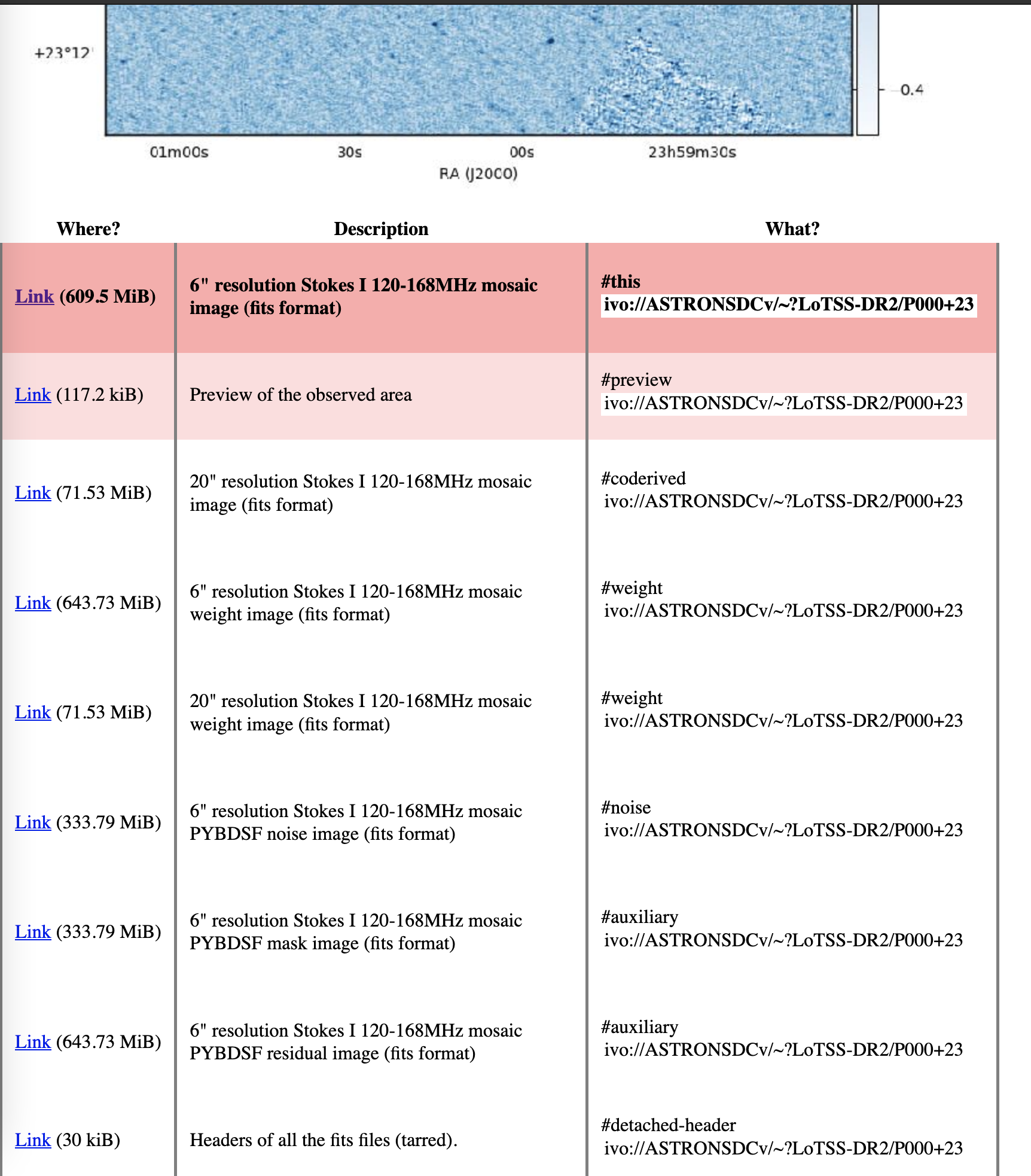
Fig. 3 Links to data products related to the target of interest. The top two items represent the primary data product (ie the one that can be directly downloaded from the main result view) and a link to the thumbnail of that data product. The other products are the anciliary data. Click for a bigger image. Note that the number of related products is too long to fit readably in a single screen shot. Click for a bigger image.
One special service is the ADQL query service, shown on Fig 4.. This contains a single box that can be used to provide custom queries using the Astronomical Data Query Language (ADQL), which in essence is a dialect of SQL. Some more information on, and examples of ADQL can be found further below.
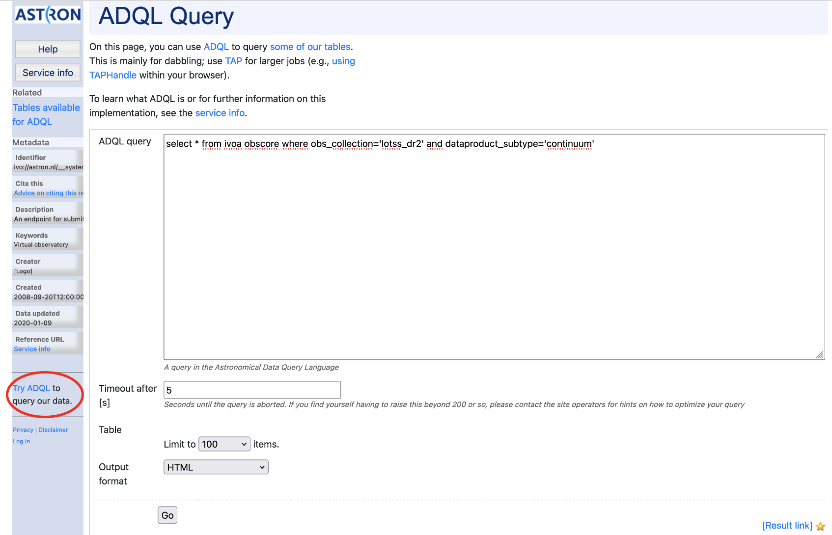
Fig. 4 ADQL query form. Click for a bigger image.
Using the DaCHS interface can be useful for users but the advantage of using a standard is that generic tooling can be used to query and access the data. Two very well-known tools are TOPCAT and Aladin. We will give an overview
Access via TOPCAT
The VO data collections can easily be accessed using TOPCAT, an interactive graphical viewer and editor for tabular data. Since the ASTRON VO is registered to the so-called registry of registries, TOPCAT can find the relevant services in its query menus. In the VO menu of TOPCAT you can pick the SIA query menu item, which will bring up a form as shown in Fig. 5. When selecting one of the data collections the SIA URL will be automatically filled in. One can then either type coordinates, or an object name and click the "Resolve" button which uses Simbad to obtain coordinates for that object. When clicking OK, a table of the data products found will appear in the main TOPCAT window. Alternatively, the table can be saved in various formats and used locally with other programs (e.g. python scripts etc).
|
|


Fig. 5: SIAP query form in TOPCAT (menu on the left), querying for data collections with LOFAR in the description, and querying for 15 arc seconds around IC 708 in LoTSS-DR1. Click for a bigger image.
Access to the tables (and the observant reader may realise here that the image data is also tabulated) in the ASTRON VO can be done using the TAP standard. The way to do this is very similar to SIA. First select TAP in the VO menu. Then you will see a list of registered TAP services. You can query those by keyword. The most obvious keyword to use to find the ASTRON VO is ASTRON. Click the Find Services and the URL will be filled in the TAP URL box. Clicking the Use Service button brings you to a window that shows a list of all the tables in the data centre and a box in which you can type ADQL. Clicking the Examples button gives you several example queries you can use to find data. In the example in Fig. 6 we are querying for the first 1000 items from tne ivoa.obscore table (which is the table that contains information on all data products in the ASTRON VO). Running the query will, again, result in a table in the the TOPCAT main window.
|
|
|
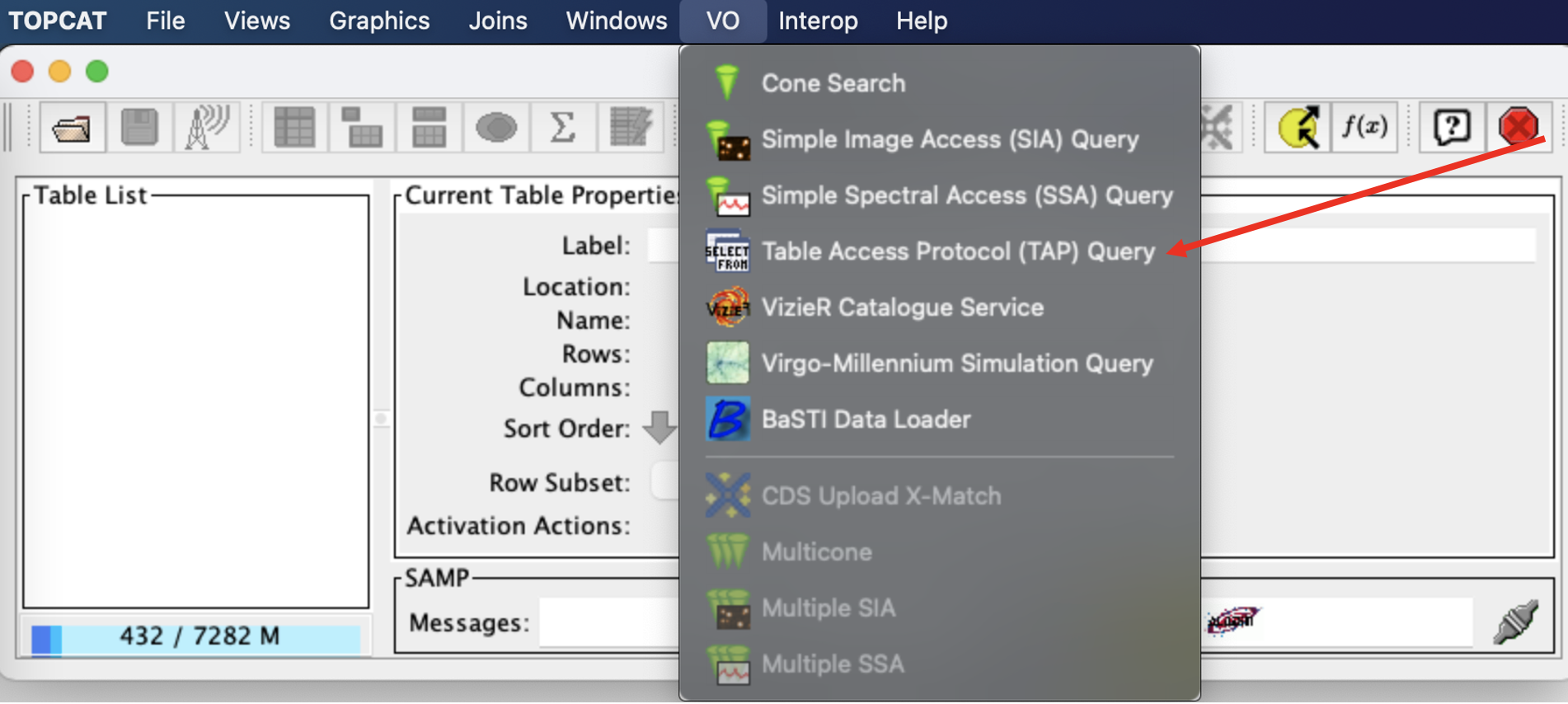
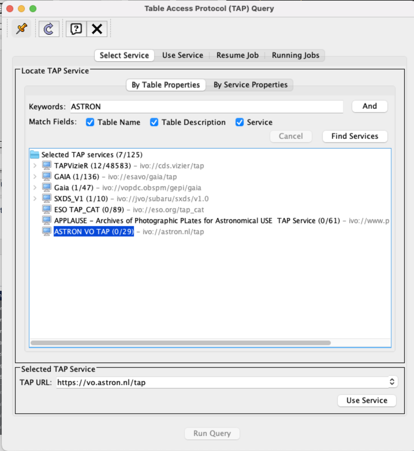
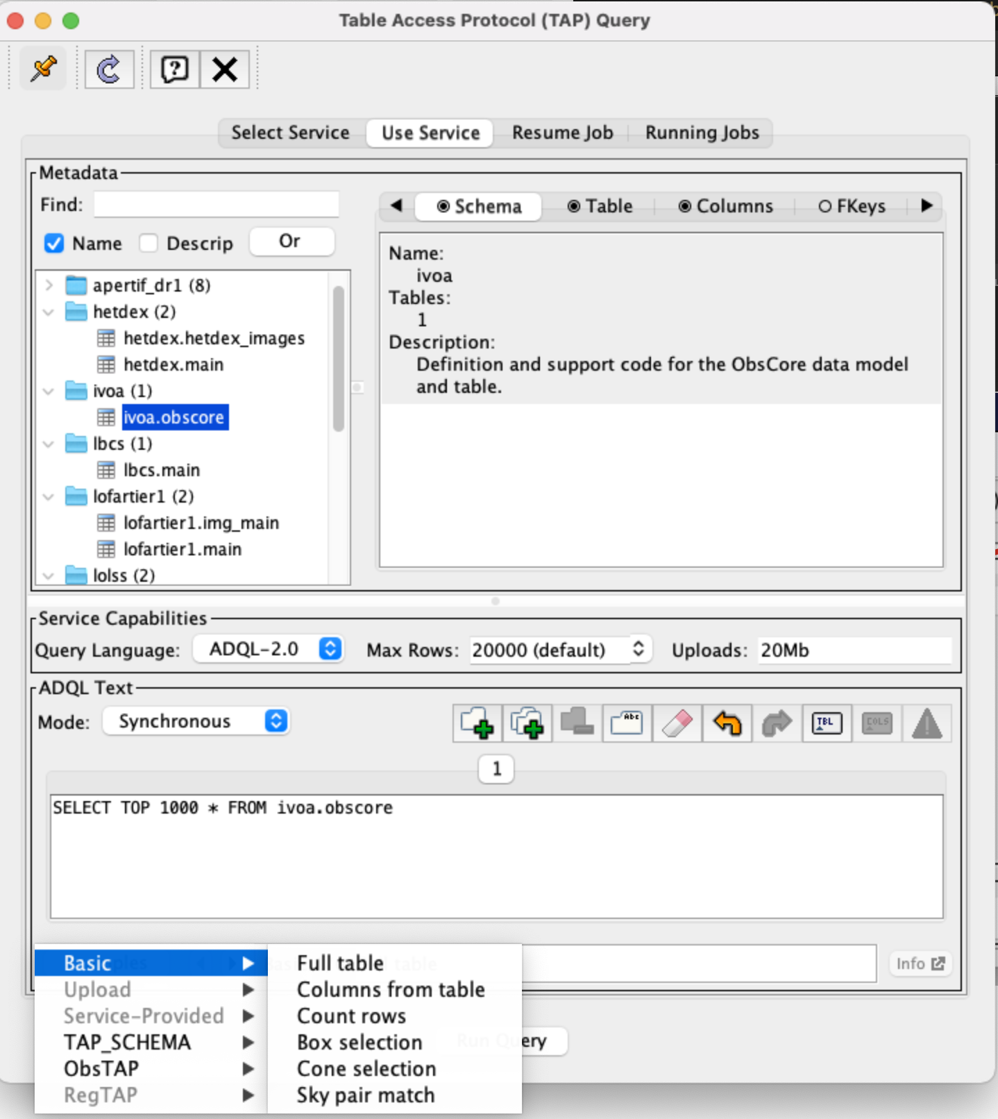
Fig. 6: TAP query form in TOPCAT (menu on the left), finding ASTRON VO (in the middle) and querying one table (in this case the obscore) using the Full table example query (on the right). Click for a bigger image.
TOPCAT and SAMP
If you have found data in the DACHS web overview, and you have TOPCAT open, you can press the Send via SAMP on the results page (see Fig. 2). When you do this, the table will automatically appear in TOPCAT. Click on the new entry as shown by the arrow in Fig. 7. At this point the table browser will open showing the content of the DACHS results). From here any TOPCAT tool can be used for further inspection and analysis of the results.
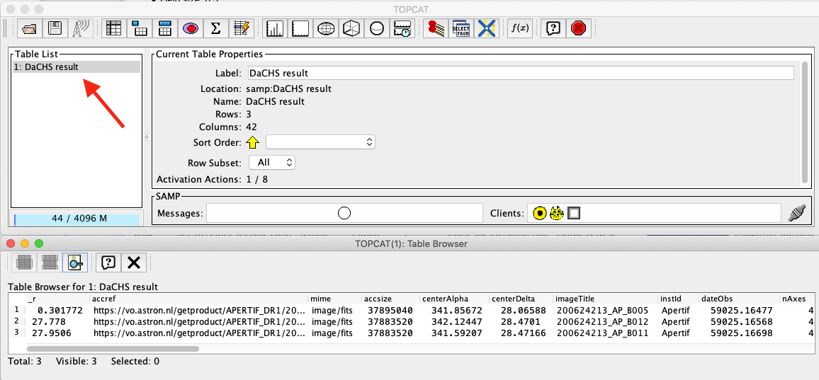
Fig.7 TOPCAT table browser view of a collection table. Click for a bigger image.
When making selections in TOPCAT, you can broadcast the resulting table using SAMP. For example Aladin will then read the table and load it in the main interface. To do this, start Aladin and push the button with the antenna indicated in Fig 8. You will see the table appear as one of the layers in Aladin.
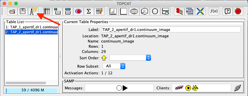
Fig. 8 How to transfer the TOPCAT query results to another VO SAMP supporting tool like ALADIN. Click for a bigger image.
Access via Aladin
One of the most popular tools to access data through the VO is Aladin Sky Atlas. There are both a browser and standalone desktop edition. When referring to Aladin in the following, this will apply to the desktop edition. Aladin is a tool that makes it possible to visualise tables and images and perform some analysis on them.
HiPS
Because the ASTRON VO has been registered with a central registry, all HiPS data collections can be visualised through Aladin. However, some of our collections have been "promoted" by the Aladin admins, and they show up at a different place in the menu structure. The promoted collections are shown in the HiPS overview at the top of this page. To bring up a HiPS, either select the Image → Radio entry in the menu (yellow directory icons) where you can see the promoted collections, or the Others → HiPS → astron.nl (purple directory icons). Alternatively you can use the select box to (partially) type the name of the HiPS you want in the background. Fig. 9 shows the HiPS of LoTSS DR1 image, and the list of ASTRON HiPSes and where to find them (please note that for presentational purposes only the ASTRON data is displayed in this screen shot).

Fig. 9 Aladin display panel. In the left column (pointed at by the red arrow) the ASTRON HiPS services are shown, witg LoTSS DR2 (high-resolution) shown. The middle panel shows the HiPS of this survey. In the right column is the "stack" which shows the loaded data sets (in this case only LoTSS DR1). Click for a bigger image.
Images
The SIA and TAP services are also available directly from Aladin. First of all, load a HiPS (any HiPS will do; but it may be useful to use the HiPS from the same data release). To find the images, you can select Others → SIA → astron.nl → <data collection name> (purple directory icons). When double-clicking the collection (or clicking the Load button) the popup screen. On top of the HiPS image, small shapes will appear that each represent the central pointing of each of the images (see Fig. 10; left). Note that the default colour of the shapes is red but the colour in the screenshot has been changed for contrast. When clicking one of the shapes the meta data of the selected object appears in a table below the figure and clicking on the image URL will then initiate a download of the original image, superimposing it on top of the HiPS (Fig. 10; right). Note that the stack on the right of the Aladin screen shows all loaded layers and that the layer in which the image was loaded is showing the percentage of the image loaded.
|
|
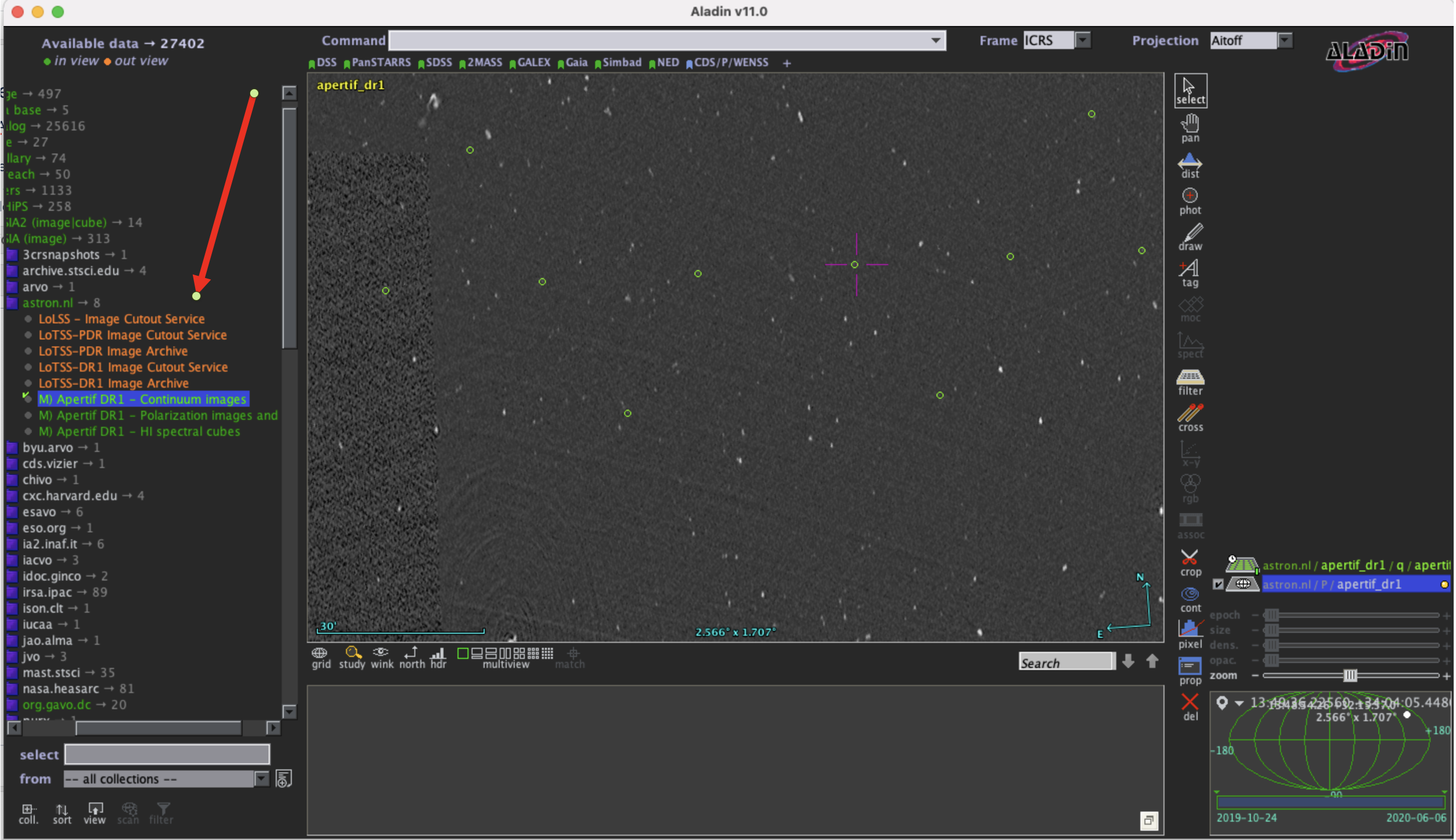
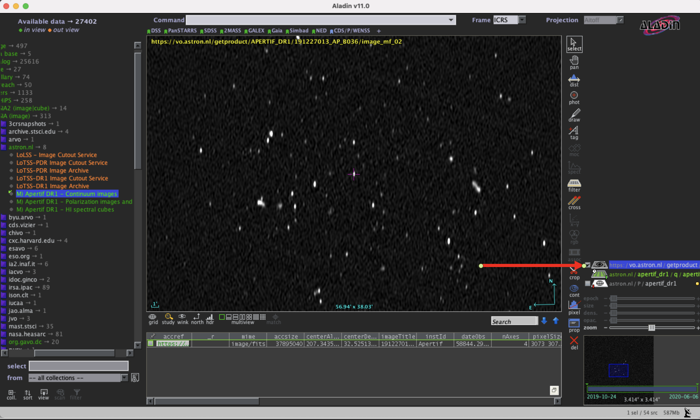
Fig. 10 Selection of one of the ASTRON SIA services. Left shows the SIA services that are available. The image panel shows the Apertif DR1 HiPS and the central pointings of the images that can be downlaoded. When downloading an image (right image), it appears on the stack and is visible in Aladin. Click for a bigger image
Catalogues
Access to catalogues through TAP is handled in a way comparable to images through SIA. Open ALADIN and on the left panel for SIAP: select Others → CS → astron.nl → <data collection name> (purple directory icons). A pop-up window will open. Click load. Note that "in view" is clicked bu default, meaning that the source in view are being loaded by default. Also note that if the Field of View is too large, the loading may fail because of a overflow on the server side (ie the query resulted in too many results). After loading, each of the catalogue entries is superimposed on top of the HiPS image as, again, a small red circle (and again this colour has been changed in the screenshot for contrast). You can then click the "select" button and select several sources (by drawing a rectangle around them) and the table of properties will appear beneath the HiPS. See Fig. 11 for a view of those steps.

Fig. 11 Aladin with LoTSS DR1 as background HiPS, superimposed the cross-matched source list. The bottom shows the properties of some of tje the sources that were manually selected.
ADQL
In several places, ADQL was mentioned as a way to construct queries to the data and catalogues. ADQL is a query language resembling SQL, so the main concepts are familiar to those acquainted with SQL. The full reference documentation (i.e. standard definition) contains all possible commands. Here we show some simple examples of table queries. You can perform queries using ADQL on the ADQL form (see Fig. 4), or for instance in TOPCAT (see Fig. 6). Also note that TOPCAT has some built in examples implemented.
In the following examples, we will follow the common practice to write SQL commands in upper case, and names of objects (tables, columns, etc) in lower case letters. The SQL commands are however case insensitive so you are totally free to for instance write select instead of SELECT.
Basic examples
The first example is simply selected all items from the lcbsw.main table:
SELECT * FROM lbcs.main
In general though, we'd like to SELECT items from a table that match certain requirements. For this we use the WHERE clause
SELECT * FROM lbcs.main WHERE baselinequal ='XXX-XXX-X'
We could add an extra requirement, for instance on the observation quality, using the AND construct:
SELECT * FROM lbcs.main WHERE baselinequal ='XXX-XXX-X' AND obsqual=15
Another useful command is DISTINCT which can be used to list distinct entries in a table. A good example of this is to list all the data collections, of which the identifier is stored in the obs_collection variable in the obscore table:
SELECT DISTINCT(obs_collection) FROM ivoa.obscore
In some cases, you may want to combine data from different tables. This can been done using so-called JOINs. The trick here is to tell the system what column in what table needs to be used to join ON.
SELECT TOP 10 * FROM apertif_dr1.continuum_images data JOIN apertif_dr1.flux_cal_visibilities flux_cal on data.obsid=flux_cal.used_for
This means that we want the first 10 entries FROM the apertif_dr1.continuum_images table, which we will call data further on in the query to save us from making typos, which should be linked to the data in the apertif_dr1.flux_cal_visibilities, which we call flux_cal, and tell it that the link should happen for each data set that appears in both and for which the obsid value in the data table is the same as the used_for value in the flux_cal table.
Export machine readable table from Apertif DR1
With everything we learned till now, we can start constructing complex queries. One good example of this is the query to obtain all the data in Apertif DR1. This query is specific to the continuum_images data product but can be adapted to other (beam-based, processed) data products by replacing the table name, e.g., for polarization cubes/images use pol_cubes.
select data.*,
flux_cal.obsid as flux_calibrator_obs_id,
pol_cal.obsid as pol_calibrator_obs_id  from apertif_dr1.continuum_images data
join  apertif_dr1.flux_cal_visibilities flux_cal on data.obsid=flux_cal.used_for and data.beam_number=flux_cal.beam
join apertif_dr1.pol_cal_visibilities pol_cal on data.obsid=pol_cal.used_for and data.beam_number=pol_cal.beam
order by obsid
Python access
The data collection and the table content can be accessed directly via python using the pyvo library. Working directly in python the tables and the data products can be simply queried and outputs can be customized according to the user’s needs, without the involvement of TOPCAT or ALADIN.
An example of a SIA query and image download can be found in the python script below (it has been tested for python 3.7). The result of the query can also be plotted using python.
#To start you have to import the library pyvo (it is also possible to use astroquery if you want)
import pyvo

## Now we will query for the LoTSS PDR SIA service at ASTRON
sia_services = pyvo.registry.search(keywords='LoTSS PDR', servicetype='sia')

## This will return two services: the cutout, and the images. We want the second item in the list so:
vo_siap_service = sia_services[1]

## If we actually know the VO identifier of the service we want to query we could also do
from pyvo.registry.regtap import ivoid2service
vo_siap_service = ivoid2service('ivo://astron.nl/lofartier1/q_img/imgs')[0]

## And now we can query for all images that cover a specific point on the sky
all_images = vo_siap_service.search(pos=(171.1, 49.6))

## So let's see what the columns of our result are:
print("Columns of the result:")
for field in all_images.fielddescs:
  print(f"name: {field.name} - units: {field.unit}")

## all_images should be sorted by distance so we pick the first for plotting. So let's grab the first one and load it in memory
hdulist = all_images[0].getdataobj()
# this may take a while for the file to download...

from astropy.wcs import WCS
import matplotlib.pyplot as plt
from matplotlib import colors

hdu = hdulist[0]  # we take the first hdu from the FITS
wcs = WCS(hdu.header)
wcs = wcs.dropaxis(2).dropaxis(2) # axis 2 of the WCS is polarisation and we are not interested in that here
plt.subplot(projection=wcs)
plt.imshow(hdu.data[0,0, 5000:7000,5000:7000], norm=colors.LogNorm(vmin=0.005), cmap='gray_r')
plt.xlabel('RA')
plt.ylabel('DEC')
plt.show()
Of course one could also use TAP to find the data using ADQL, download the file and imaging it, For Apertif DR1 it would look like this
## To perform a TAP query you have to connect to the service first
tap_service = pyvo.dal.TAPService('https://vo.astron.nl/__system__/tap/run/tap')

# This works also for
from pyvo.registry.regtap import ivoid2service
vo_tap_service = ivoid2service('ivo://astron.nl/tap')[0]

# The TAPService object provides some introspection that allow you to check the various tables and their
# description for example to print the available tables you can execute
print('Tables present on http://vo.astron.nl')
for table in tap_service.tables:
 print(table.name)
print('-' * 10 + '\n' * 3)

# or get the column names
print('Available columns in apertif_dr1.continuum_images')
print(tap_service.tables['apertif_dr1.continuum_images'].columns)
print('-' * 10 + '\n' * 3)

## You can obviously perform tap queries accross the whole tap service as an example a cone search
print('Performing TAP query')
result = tap_service.search(
 "SELECT TOP 5 target, beam_number, accref, centeralpha, centerdelta, obsid, DISTANCE(" \
     "POINT('ICRS', centeralpha, centerdelta),"\
     "POINT('ICRS', 208.36, 52.36)) AS dist"\
 " FROM apertif_dr1.continuum_images"  \
 " WHERE 1=CONTAINS("
 "    POINT('ICRS', centeralpha, centerdelta),"\
 "    CIRCLE('ICRS', 208.36, 52.36, 0.08333333)) "\
 " ORDER BY dist ASC"
 )
print(result)

# The result can also be obtained as an astropy table
astropy_table = result.to_table()
print('-' * 10 + '\n' * 3)

## You can also download and plot the image
import astropy.io.fits as fits
from astropy.wcs import WCS
import matplotlib.pyplot as plt
import requests, os
import numpy as np

# DOWNLOAD only the first result
#
print('Downloading only the first result')
file_name = '{}_{}_{}.fits'.format(
 result[0]['obsid'].decode(),
 result[0]['target'].decode(),
 result[0]['beam_number'])
path = os.path.join(os.getcwd(), file_name)
http_result = requests.get(result[0]['accref'].decode())
print('Downloading file in', path)
with open(file_name, 'wb') as fout:
 for content in http_result.iter_content():
     fout.write(content)
hdu = fits.open(file_name)[0]
wcs = WCS(hdu.header)
# dropping unnecessary axes
wcs = wcs.dropaxis(2).dropaxis(2)
plt.subplot(projection=wcs)
plt.imshow(hdu.data[0, 0, :, :], vmax=0.0005)
plt.xlabel('RA')
plt.ylabel('DEC')
plt.show()
Overview
Content Tools
Tasks